A while back I found myself in the need of an adjustable RF attenuator capable of high-GHz operation. As luck would have it I had an old Spectrum analyser on the shelf at work, which we had retired quite some time ago.
Spectrum analysers being quite capable test instruments, I knew that the input attenuation would be done with a standalone module that we could recover for reuse without too much trouble.
The attenuator module
Here’s the module itself, with the factory drive PCB removed from the bottom, showing the solenoids that operate the RF switches. There are test wires attached to them here to work out which solenoid switches which attenuation stage. In the case of this module, there are switches for the following:
Input select switch
AC/DC coupling
-5dB
-10dB
-20dB
-40dB
For me this means I have up to -75dB attenuation in 5dB steps, with optional switchable A-B input & either AC or DC coupling.
Drive is easy, requiring a pulse on the solenoid coil to switch over, the polarity depending on which way the switch is going.
Building a Control Board
Now I’ve identified that the module was reusable, it was time to spin up a board to integrate all the features we needed:
Onboard battery power
Pushbutton operation
Indication of current attenuation level
The partially populated board is shown at right, with an Arduino microcontroller for main control, 18650 battery socket on the right, and control buttons in the centre. The OLED display module for showing the current attenuation level & battery voltage level is missing at the moment, but it’s clear where this goes.
As there weren’t enough GPIO pins for everything on the Arduino, a Microchip MC23017 16-Bit I/O expander, which is controlled via an I²C bus. This is convenient since I’m already using I²C for the onboard display.
Driving the Solenoids
A closer view of the board shows the trip of dual H-Bridge drivers on the board, which will soon be hidden underneath the attenuator block. These are LB1836M parts from ON Semiconductor. Each chip drives a pair of solenoids.
Power Supplies
The bottom of the board has all the power control circuitry, which are modularised for ease of production. There’s a Lithium charge & protection module for the 18650 onboard cell, along with a boost converter to give the ~9v rail required to operate the attenuator solenoids. While they would switch at 5v, the results were not reliable.
Finishing off
A bit more time later, some suitable firmware has been written for the Arduino, and the attenuator block is fitted onto the PCB. The onboard OLED nicely shows the current attenuation level, battery level & which input is selected.
Here’s one of the old modems from my spares bin, a Vodafone Mobile WiFi R207. This is just a rebranded Huawei E5330. This unit includes a 3G modem, and a WiFi chipset, running firmware that makes this a mini-router, with NAT.
Specs
The back has the batter compartment & the SIM slot, with a large label showing all the important details.
Cover Removed
A couple of small Torx screws later & the shell splits in half. All the electronics are covered by shields here, but luckily they are the clip-on type, and aren’t soldered direct to the PCB.
Chipset
Once the shield has been removed, the main chipset is visible underneath. There’s a large Spansion MS01G200BHI00 1GBit flash, which is holding the firmware. Next to that is the Hi6758M baseband processor. This has all the hardware required to implement a 3G modem. Just to the right is a Hi6521 power management IC, which is dealing with all the power supplies needed by the CPU.
The RF section is above the baseband processor, some of which is hiding under the bits of the shield that aren’t removable.
SIM Socket
There’s a socket onboard for a standard Mini-SIM, just to the left of that is a Hi6561 4-phase buck converter. I would imagine this is providing the power supplies for the RF section & amplifier.
Unpopulated Parts
Not sure what this section is for, all the parts are unpopulated. Maybe a bluetooth option?
PCB Reverse
The other side of the PCB is pretty sparse, holding just the indicator LEDS, button & the WiFi Chipset.
Realtek WiFi Chipset
The chipset here is a Realtek part, but it’s number is hidden by some of the shield. The antenna connection is routed to the edge of the board, where a spring terminal on the plastic case mounted antenna makes contact.
Time for more silicon pr0n! When Virgin Media supplied me with a new modem, they requested I “recycle” the old one, so naturally it got gutted for the component parts. This particular IC is the frontend of the RF tuner. Unfortunately no datasheet is available, but I did manage to find some info in a press release. The sections are clearly identifiable, the RF section is on the left, while the rest of the demodulating logic is hidden on the right under a metal layer.
MXL261 Die – Click to Embiggen!
The MxL261 is based on MaxLinear’s low-power, digital CMOS process RF and mixed-signal technology. It is a single-die, global standards, digital cable front end with integrated splitter, two 100MHz wideband tuners, four QAM demodulators and a four-channel-wide IF output.
Here’s another Sony Flat CRT TV, the FD0280. This one was apparently the last to use CRT technology, later devices were LCD based. This one certainly doesn’t feel as well made as the last one, with no metal parts at all in the frame, just moulded plastic.
CRT Screen
Being a later model, this one has a much larger screen.
Autotuning
Instead of the manual tuner of the last Watchman, this one has automatic tuning control, to find the local stations.
Spec Label
The spec puts the power consumption a little higher than the older TV, this isn’t surprising as the CRT screen is bigger & will require higher voltages on the electrodes.
Certification Label
The certification label dates this model to May 1992.
External Inputs
Still not much in the way of inputs on this TV. There’s an external power input, external antenna input & a headphone jack. No composite from the factory. (Hack incoming ;)).
Power / Band
The UHF/VHF & power switches are on the top of this model.
Back Cover Removed
Removing some very tiny screws allows the back to be removed. There’s significant difference in this model to the last, more of the electronics are integrated into ICs, nearly everything is SMD.
RF Section
There’s the usual RF tuner section & IF, in this case the VIF/SIF is a Mitsubishi M51348AFP.
Tuner Controller
The digital control of the tuner is perfomed by this Panasonic AN5707NS.
Deflection / Sync
The deflection & sync functions appear to be controlled by a single Sony branded custom IC, the CX20157. Similar to many other custom Sony ICs, a datasheet for this wasn’t forthcoming.
PCB Top
There’s very little on the top side of the board, the RF section is on the left, there’s a DC-DC converter bottom centre next to the battery contacts. This DC-DC converter has a very unusual inductor, completely encased in a metal can. This is probably done to prevent the magnetic field from interfering with the CRT.
CRT
Here’s the CRT itself, the Sony 03-JM. The back of this CRT is uncoated at the bottom, the tuning scale was taped to the back so it lined up with the tuning bar displayed on the screen.
Electronics
Here’s the electronics completely removed from the shell. There’s much more integration in this model, everything is on a single PCB.
Phosphor Screen
The curve in the phosphor screen can clearly be seen here. This CRT seems to have been cost-reduced as well, with the rough edges on the glass components having been left unfinished.
Electron Gun
Here’s the electron gun end of the tube. There isn’t a separate final anode connection to the bell of the tube unlike the previous model. Instead the final anode voltage is on a pin of the electron gun itself. This keeps all the wiring to the tube at one end & shortens the high voltage cable.
Electron Gun
Here’s the gun in the neck of the tube. Again this is pretty much standard fare for CRT guns. It’s more similar to a viewfinder tube in that the anode connection is running from the pins at the back. (It’s the line running up the right side of the tube). I’m guessing the anode voltage is pretty low for this to work without the HV flashing over, probably in the 2-4kV range.
Hacking the Sony FD-20 to accept a composite input is easy – the tuner receives the RF transmission, produces an IF, this is then fed into IC201, a Mitsubishi M51364P Video IF Processor. The VIF IC then separates out the composite video signal, which is output on Pin 13 (in photo above, left side, 3rd pin from the top). The audio is separated out & sent via Pin 11 to the Audio IF processor.
In the above photo, the VIF IC has been removed from the board with hot air, as it was interfering with the signal if left in place. The RF tuner was also desoldered & removed. Unfortunately I managed to mangle a pad, which is the ground pin for the VIF IC. This isn’t much of an issue though, as an identical signal ground is available, just to the left of the IC.
Audio Input
The audio can be tapped into in a similar way, the circled pad in the centre of the photo marked SIF is the place, this is the output of the Audio IF processor to the audio amplifier. The Audio IF processor didn’t interfere with the injected signal, so it was left in place.
The term laser stands for “Light Amplification by Stimulated Emission of Radiation”. However, lasers as most of us know them, are actually sources of light – oscillators rather than amplifiers. (Although laser amplifiers do exist in applications as diverse as fibre optic communications repeaters and multi-gigawatt laser arrays for inertial fusion research.) Of course, all oscillators – electronic, mechanical, or optical – are constructed by adding the proper kind of positive feedback to an amplifier.
All materials exhibit what is known as a bright line spectra when excited in some way. In the case of gases, this can be an electric current or (RF) radio frequency field. In the case of solids like ruby, a bright pulse of light from a xenon flash lamp can be used. The spectral lines are the result of spontaneous transitions of electrons in the material’s atoms from higher to lower energy levels. A similar set of dark lines result in broad band light that is passed through the material due to the absorption of energy at specific wavelengths. Only a discrete set of energy levels and thus a discrete set of transitions are permitted based on quantum mechanical principles (well beyond the scope of this document, thankfully!). The entire science of spectroscopy is based on fact that every material has a unique spectral signature.
The HeNe laser depends on energy level transitions in the neon gas. In the case of neon, there are dozens if not hundreds of possible wavelength lines of light in this spectrum. Some of the stronger ones are near the 632.8 nm line of the common red HeNe laser – but this is not the strongest:
The strongest red line is 640.2 nm. There is one almost as strong at 633.4 nm. That’s right, 633.4 nm and not 632.8 nm. The 632.8 nm one is quite weak in an ordinary neon spectrum, due to the high energy levels in the neon atom used to produce this line.
Bright Line Spectra of Helium and Neon
(The relative brightnesses of these don’t appear to be accurate though at present.) More detailed spectra can be found at the: Laser Stars – Spectra of Gas Discharges Page. And there is a photo of an actual HeNe laser discharge spectra with very detailed annotation of most of the visible lines in: Skywise’s Lasers and Optics Reference Section. The comment about the output wavelength not being one of the stronger lines is valid for most lasers as if it were, that energy level would be depleted by spontaneous emission, which isn’t what is wanted!
There are also many infra-red lines and some in the orange, yellow, and green regions of the spectrum as well.
The helium does not participate in the lasing (light emitting) process but is used to couple energy from the discharge to the neon through collisions with the neon atoms. This pumps up the neon to a higher energy state resulting in a population inversion meaning that more atoms in the higher energy state than the ground or equilibrium state.
Helium-Neon Excitation and Lasing Process
It turns out that the upper level of the transition that produces he 632.8 nm line (as well as the other visible He-Ne lasing lines) has an energy level that almost exactly matches the energy level of helium’s lowest excited state. The vibrational coupling between these two states s highly efficient.
A DC electrical discharge or RF field excites He atoms to the 2s energy state.
Collisions efficiently transfer energy raising Ne atoms to the 3s2 energy state. Note the relatively high energy levels involved – over 20 eV for the upper energy states.
Stimulated emission (lasing) causes a drop to one of several Ne 2p states.
Radiative decay (spontaneous emission) drops Ne from the terminal lasing state to the 1s state.
Collisions with the tube wall drops Ne from the 1s state to the Ground state.
For 632.8 nm, one mirror will be highly reflective at 632.8 nm (typically 99.9 percent or better). This is the “High Reflector” or HR. The other mirror will have a typical reflectivity of 99 percent at 632.8 nm. This is the “Output Coupler” or OC from which the useful beam emerges. In order to suppress lasing at other wavelengths, the mirrors will generally be designed to have lower reflectivity there. (Though given the low gain of all the He-Ne lasing lines, especially the “other colour” lines, this isn’t much of a problem at 632.8 nm.)
The rate at which (4) and (5) can take place ultimately limits the power of a He-Ne laser and explains why increasing the excitation (1) actually reduces power above some optimum level.
The gas mixture must be mostly helium (typically 5:1 to 10:1, He:Ne), so that helium atoms can be excited. The excited helium atoms collide with neon atoms, exciting some of them to the state from which they can radiate at 632.8 nm. Without helium, the neon atoms would be excited mostly to lower excited states responsible for non-laser lines. And the gas mixture has to be super pure as any contamination results in excitation of rogue atoms (like H, O, and N) to lower energy states where all that will happen is that they will glow like a poorly made neon sign.
A neon laser with no helium can be constructed but it is much more difficult and the output power will be much lower without this means of energy coupling. Therefore, a He-Ne laser that has lost enough of its helium (e.g., due to diffusion through the seals or glass) will most likely not lase at all since the pumping efficiency will be too low.
However, pure neon will lase superradiantly in a narrow tube (e.g., 40 cm long x 1 mm ID) in the orange (611.9 nm) and yellow (594.1 nm) with orange being the strongest. Superradiant means that no mirrors are used although the addition of a Fabry-Perot cavity (e.g., mirrors!) does improve the lateral coherence and output power. This from a paper entitled: “Super-Radiant Yellow and Orange Laser Transitions in Pure Neon” by H. G. Heard and J. Peterson, Proceedings of the IEEE, Oct. 1964, vol. #52, page #1258. The authors used a pulsed high voltage power supply for excitation (they didn’t attempt to operate the system in CW mode but speculate that it should be possible).
(From: Steve Roberts.)
“Various IR lines will lase in pure neon, and even the 632.8 nm line will lase, but it takes a different pressure and a much longer tube. 632.8 nm also shows up with neon-argon, neon-oxygen, and other mixtures. Just about everything on the periodic table will lase, given the right excitation. See “The CRC Handbook of Lasers” or one of the many compendiums of lasing lines available in larger libraries. These are usually 4 volume sets of books the size of a big phone book just full of every published journal article on lasing action observed. It’s a shame that out of these many thousands and thousands of lasing lines, only 7 different types of lasers are under mainstream use.
There are many possible transitions in neon from the excited state to a lower energy state that can result in laser action. (Only the three found most commonly in commercial He-Ne lasers are shown in the diagram, above.) The most important (from our perspective) are listed below:
1
2
3
4
5
6
7
8
9
10
11
12
13
14
15
16
17
18
19
20
21
22
23
24
25
26
(1)(2)(3)(4)(5)(6)
Output HeNe Perceived Lasing Typical Maximum
Wavelength Laser Name Beam Colour Transition Gain(%/m)Power(mW)
Output Wavelength is approximate. In addition to slight variations due to actual lasing conditions (single mode, multimode, doppler broadening, etc.), some references don’t even agree on some of these values to the 4 or 5 significant digits shown.
He-Ne Laser Name is what would be likely to be found in a catalogue or spec. sheet. All those that have an entry in this column are readily available commercially.
Perceived Beam Colour is how it would appear when spread out and projected onto a white screen. Of course, depending on the revision level of your eyeballs, this may vary someone from individual to individual. 🙂
Lasing Transition uses the so-called “Paschen Notation” and indicates the electron shells of the neon atom energy states between which the stimulated emission takes place.
Typical Gain (%/m) shows the percent increase in light intensity due to stimulated emission at this wavelength inside the laser tube’s bore. This is the single pass gain and will be affected by tube construction, gas fill ratio and pressure, discharge current, and other factors. The first column is from various sources. The second column is from Hecht, “The Laser Guide Book”. However, a newer text: Mark Csele, “Fundamentals of light sources and lasers” (ISBN 0-471-47660-9, Wiley-Interscience, 2004) lists the typical gain as 1.2 to 1.5 at 633 nm. And measurements by myself and others seem to show that this slightly higher value may be more accurate, at least under some conditions.
Gain at 1,523 nm may be similar to that of 543.5 nm – about 0.5%/m. Gain at 3,391 nm is by far the highest of any – possibly more than 100%/m. I know of one particular He-Ne laser operating at this wavelength that used an OC with a reflectivity of only 60% with a bore less than 0.4m long. Yet, the output power of the largest 3,391 nm commercial He-Ne laser is still only a fraction of that at 632.8 nm.
Maximum Power shows the highest output power lasers commercially available in a TEM00 beam for each wavelength. The first number is rated power while the number in () is achieved output power for a particularly lively tube. Lasers operating with multiple (spatial) modes (non-TEM00) may have somewhat higher output power.
The most common and least expensive He-Ne laser by far is the one called ‘red’ at 632.8 nm. However, all the others with named ‘colours’ are readily available with green probably being second in popularity due to its increased visibility near the peak of the of the human eye’s response curve (555 nm). And, with some He-Ne lasers with insufficiently narrow-band mirrors, you may see 640 nm red as a weak output along with the normal 632.8 nm red because of its relatively high gain. There are even tunable He-Ne lasers capable of outputting any one of up to 5 or more wavelengths by turning a knob. While we normally don’t think of a He-Ne laser as producing an infra-red (and invisible) beam, the IR spectral lines are quite strong – in some cases more so than the visible lines – and He-Ne lasers at all of these wavelengths (and others) are commercially available.
The first gas laser developed in the early 1960s was an HeNe laser operated at 1,152.3 nm. In fact, the IR line at 3,391.3 is so strong that a HeNe laser operating in ‘superradiant’ mode – without mirrors – can be built for this wavelength and commercial 3,391.3 nm HeNe lasers may use an output mirror with a reflectivity of less than 50 percent. Contrast this to the most common 632.8 nm (red) He-Ne laser which requires very high reflectivity mirrors (often over 99 percent) and extreme care to minimize losses or it won’t function at all.
When the He-Ne gas mixture is excited, all possible transitions occur at a steady rate due to spontaneous emission. However, most of the photons are emitted with a random direction and phase, and only light at one of these wavelengths is usually desired in the laser beam. At this point, we have basically the glow of a neon sign with some helium mixed in!
To turn spontaneous emission into the stimulated emission of a laser, a way of selectively amplifying one of these wavelengths is needed and providing feedback so that a sustained oscillation can be maintained. This may be accomplished by locating the discharge between a pair of mirrors forming what is known as a Fabry-Perot resonator or cavity. One mirror is totally reflective and the other is partially reflective to allow the beam to escape.
One mirror may be perfectly flat (planar) or both may be spherical with a typical Radius of Curvature (RoC = 2 * focal length) slightly longer that the length of the cavity (L) or even longer. Where both mirrors have an RoC equal to L, the configuration is called ‘confocal’ (the focii of the two mirrors are coincident), but it is marginall stable, so the RoCs will be at least slightly longer than L. A cavity with two planar mirrors is borderline stable and essentially impossible to align or maintain in alignment over time, so it is never used in He-Ne lasers (but is in some pulsed solid state and other lasers). Curved mirrors result in an easier to align more stable configuration but are more expensive than planar mirrors to manufacture and are not as efficient since less of the lasing medium volume is used (think of the shape of the beam inside the bore). The confocal arrangement represents a good compromise between a true spherical cavity (r = 1/2 * L) which is easiest to align but least efficient and one with plane parallel mirrors (f = infinity) which is most difficult to align but uses the maximum volume of the lasing medium. (But as noted above, for a practical confocal cavity, RoCs slightly longer than L are used to assure stability.)
These mirrors are normally made so that the two mirrors together has peak reflectivity at the desired laser wavelength. (For technical reasons, it’s sometimes easier to make mirrors like cliffs – high reflectivity that drops to low reflectivity at a given wavelength, in either direction – than to guarantee a particular peak reflectivity.) When a spontaneously emitted photon resulting from the transition corresponding to this peak happens to be emitted in a direction nearly parallel to the long axis of the tube, it stimulates additional transitions in excited atoms. These atoms then emit photons at the same wavelength and with the same direction and phase. The photons bounce back and forth in the resonant cavity stimulating additional photon emission. Each pass through the discharge results in amplification – gain – of the light. If the gain due to stimulated emission exceeds the losses due to imperfect mirrors and other factors, the intensity builds up and a coherent beam of laser light emerges via the partially reflecting mirror at one end. With the proper discharge power, the excitation and emission exactly balance and a maximum strength continuous stable output beam is produced.
Spontaneously emitted photons that are not parallel to the axis of the tube will miss the mirrors entirely or will result in stimulated photons that are reflected only a couple of times before they are lost out the sides of the tube. Those that occur at the wrong wavelength will be reflected poorly if at all by the mirrors and any light at these wavelengths will die out as well.
Summary of the He-Ne Lasing Process
The He-Ne laser is a 4 level laser (see the table above for the specific energy level transitions for the common wavelengths):
Collisions with excited helium atoms raise the neon atoms from level 1 (ground state) to level 4 (which is the 3s state for visible wavelengths).
The visible lasing transitions are from the 3s to various 2p states (depending on wavelength) or level 3.
The neon atoms then decay rapidly to the 1s state or level 2.
Return to the ground state or level 1 is aided by collisions with the He-Ne laser tube’s bore/capillary walls.
For most common IR wavelengths, level 4 is the 2s state and level 3 are various 2p states. However, the very strong 3.93 um line originates from the 3s state just like the visible wavelengths – and is the reason it competes with them in long He-Ne tubes and must be suppressed to optimize visible output.
The ‘s’ states of neon have about 10 times the lifetime of the ‘p’ states and thus support the population inversion since a neon atom can hang around in the 2s state long enough for stimulated emission to take place. However, the limiting effect is the decay back to level 1, the ground state, since the 1s state also has a long lifetime. Thus, one wants a narrow bore to facilitate collisions with its walls. But this results in increased losses. Modern He-Ne lasers operate at a compromise among several contradictory requirements which is one reason that their maximum output power is relatively low.
Approximate Reference Values for the Red (632.8 nm) He-Ne Laser
Here are some common values and relationships that may come in handy when doing calculations. These are not the most exact since they may depend on other factors like the precise gas-fill and environmental conditions but are generally good enough for government work. 🙂
Wavelength: 632.8 nm.
Optical Frequency: 474 THz.
Gain Bandwidth of Neon: 1.6 GHz or 2.136 nm.
1 nm at 632.8 nm: 749 GHz.
1 GHz at 632.8 nm: 1.335 nm.
Longitudinal Modes of Operation
The physical dimensions of the Fabry-Perot resonator impose some additional constraints on the resulting beam characteristics.
While it is commonly believed that the 632.8 nm (for example) transition is a sharp peak, it is actually a Gaussian – bell shaped – curve. (Strictly speaking, it is something called a “Voigt distribution” which is a combination of Gaussian and Lorentzian – but that’s for the advanced course. Gaussian is close enough for this discussion since the discrepancy only shows up way out in the tails of the curve.) In order for a linear or (Fabry-Perot) cavity to resonate strongly, a standing wave pattern must exist. This will only occur when an integral number of half wavelengths fit between the two mirrors. This restricts possible axial or longitudinal modes of oscillation to:
1
2
3
L *2c *n
W=---------orF=---------
nL *2
Where:
L is the distance between the mirrors (m).
W denotes the possible wavelengths of oscillation (m).
n is a large integer (order of 948,000 for W around 632.8 nm, L = .3 m).
F denotes the possible frequencies of oscillation (Hz).
c is the speed of light (approximately 300 million m/s).
The laser will not operate with just any wavelength – it must satisfy this equation. Therefore, the output will not usually be a single peak at 632.8 nm but a series of peaks around 632.8 nm spaced c/(2*L) Hz apart. Longer cavities result in closer mode spacing and a larger number of modes since the gain won’t fall off as rapidly as the modes move away from the peak. For example, a cavity length of 150 mm results in a longitudinal mode spacing of about 1 GHz; L = 300 mm results in about 500 MHz. The strongest spectral lines in the output will be nearest the combined peak of the lasing medium and mirror reflectivity but many others will still be present. This is called multimode operation.
Think of the vibrating string of a violin or piano. Being fixed at both ends, it can only sustain oscillations where an integer number of cycles fits on the string. In the case of a string, n can equal 1 (fundamental) and 2, 3, 4, 5 (harmonics or overtones). Due to the tension and stiffness of the string, only small integer values for n are present with a significant amplitude. For a He-Ne laser, the distribution of the selected neon spectral line and shape of the reflectivity function of the mirrors with respect to wavelength determine which values of n are present and the effective gain of each one. And n will be much greater than 1!
For a typical HeNe laser tube, possible values of n will form a series of very large numbers like 948,161, 948,162, 948,163, 948,164,…. rather than 1, 2, 3, 4. 🙂 A typical gain function showing the emission curve of the excited neon multiplied by the mode structure of the Fabry-Perot resonator and the reflectivity curve of the mirrors may look something like the following:
Or, see the following for some slightly more aesthetically pleasing diagrams of the longitudinal modes of random polarized He-Ne lasers. 🙂
Longitudinal Modes of Typical Random Polarized 1 mW He-Ne LaserLongitudinal Modes of Typical Random Polarized 3 mW He-Ne LaserLongitudinal Modes of Typical Random Polarized 8 mW He-Ne LaserLongitudinal Modes of Typical Random Polarized 30 mW He-Ne Laser
Mode Sweep
Since the mode locations are determined by the physical spacing of the mirrors, as the tube warms up and expands, these spectral line frequencies are going to drift downward (toward longer wavelengths). However, since the reflectivity of the mirrors as a function of wavelength is quite broad (for all practical purposes, a constant), new lines will fill in from above and the overall shape of the function doesn’t change.
In the diagrams above, a single arbitrary mode position is shown, but for well behaved lasers, the lasing lines will move smoothly through the gain curve as the laser warms up. This is called by various names including “mode sweep” and “mode cycling”. While present with most lasers, the effects are quite striking with low to medium power He-Ne lasers due to their relatively narrow neon gain bandwidth (which is only a small multiple of the longitudinal mode spacing in low to medium power He-Ne lasers), the rather fortuitous phenomenon that for red (633 nm) He-Ne lasers at least, adjacent longitudinal modes tend to be orthogonally polarized, and nearly ideal behaviour in other respects with the Physics mostly cooperating. (Murphy has seen the LASER DANGER signs and stays away!) Much more on all this below (except perhaps for Murphy).
In the nice diagram above 🙂 of the 8 mW laser, there are 5 longitudinal cavity modes that see gain above the lasing threshold (the right-most just barely). These become lasing modes (red and blue) producing a total output power of somewhat over 8 mW in this specific example. For the 30 mW laser, there are twice as many lasing modes one half the distance apart, and each mode has more power. Interestingly, adjacent modes in a so-called “random polarized” red (632.8 nm) He-Ne laser are almost always orthogonally polarized, with the polarization axes fixed relative to the tube. (Here, one of them is arbitrarily referenced as 0 degrees, more on this later). As the distance between the mirrors is increased, the number of oscillating modes increases as well, though the actual power in each mode increases only slightly.
Mode Sweep of 8 mW Random Polarized He-Ne Laser
One complete cycle (red or blue) represents a change in cavity length of one wavelength (at 633 nm) and a change in optical frequency of 2 times the mode spacing of c/2L. The additional factor of 2 arises because the adjacent modes of the red (633 nm) HeNe are orthogonally polarized. This is not true with most other lasers and even HeNe lasers at other wavelengths. Note that while the profile of the mode sweep is affected by the neon gain curve, the period is NOT directly related to it, only c/2L.
However, note that as HeNe lasers get longer, mode competition results in greater and greater instability, so don’t expect to see a nice orderly march with a Spectra-Physics 127 (39 inch cavity). In fact while the envelope of the modes will generally follow the gain curve, each mode will be jumping up and down in a quasi-chaotic dance! Instability may appear in the display of a Scanning Fabry-Perot Interferometer (SFPI) when viewing the longitudinal modes of a 633 nm HeNe with tubes rated at 7 to 10 mW. 5 mW lasers are usually quite clean while 35 mW lasers can be a real mess.
For very short HeNe tubes, the width of the gain curve may be similar to or even narrower than the spacing between modes. With those, the output power will become very low or go to zero during portions of the mode sweep. Very few HeNe lasers were produced with cavity lengths where this would be an issue since maximum output power would be very low. The only one I know of was the Spectra-Physics 119 stabilized laser with a 100 mm cavity length (mode spacing of 1.5 GHz). The very short cavity was required to provide special characteristics for this system.
In fact, it’s often possible to go so far as to identify a specific manufacturer and even model of a HeNe laser tube based solely on the plots of its polarized mode sweep, providing a sort of “fingerprint” for lasers. 🙂 For example, the type of tube installed in a Zygo or Teletrac/Axsys stabilized laser can be determined without opening the case!
He-Ne Laser Mode Sweep Fingerprints
These tubes are all physically similar yet have dramatically different mode sweep plots. And, it’s often possible to determine key information about the health of a laser tube by comparing its mode sweep with that of a new one. Over most of its life, the general shape will remain the same, but as the power declines, in addition to the total height of the plot decreasing, the amplitude of the variation (i.e., the AC component) relative to the total will increase. However, near end-of-life when power is way down and fewer modes are oscillating, the distinctions will tend to disappear.
For very long tubes like the 30 mW one in the example above where there are many longitudinal modes, the actual appearance of mode sweep may be rather chaotic as power shifts among the modes in a random dance. When I first observed this behaviour with a Melles Griot 05-LHP-928 (35 mW) He-Ne producing over 40 mW, I thought it might have been defective in some way despite the high power. But two other healthy samples behaved in a similar manner. So, don’t expect to see nice well behaved marching modes for these high power lasers. There is often a hint of instability even in shorter tubes though it may be subtle – a few percent variation in the peak amplitudes not attributable to other causes like normal movement under the gain curve or power supply ripple.
The effects of mode sweep are more dramatic with short low pressure carbon dioxide (CO2) lasers because for a given resonator length, the ratio of wavelengths (10,600 nm for CO2 compared to 632.8 nm for He-Ne means that the longitudinal mode spacing is 16.7 times larger). In these cases, the laser output will turn on and off as it heats up and the distance between the mirrors increases due to thermal expansion. For this to happen in a 632.8 nm He-Ne would require the tube to be less than about 75 mm (3 inches) in length.
A linearly polarized He-Ne laser would have the same longitudinal mode spacing, but all the lasing modes would have the same polarization orientation (red or blue) as shown in the diagrams and animations, above.
Longitudinal Modes of Typical Linearly Polarized 8 mW He-Ne Laser
So, someone with red/blue color-blindness (if there is such a thing) would see the diagrams for all them as being linearly polarized!
A label on the polarized laser will indicate the plane or orientation of polarization of the output beam. For a random polarized He-Ne laser, a polarizer oriented at 45 degrees with respect to the plane of polarization would produce an output with respect to mode sweep that is similar to that of a linearly polarized laser, except that even with an ideal polarizer, the output power would be cut in half.
Now for some actual numbers: The Doppler-broadened gain curve for neon in a red (632.8 nm) He-Ne laser has a Full Width Half Maximum (FWHM, where the gain is at least half the peak value) on the order of 1.5 or 1.6 GHz. So, for a 500 mm long (high gain) tube with its mode spacing of about 300 MHz (similar to what is depicted above), 5 or 6 lines may be active simultaneously and oscillation will always be sustained (though there would be some variation in output power as various modes sweep by and compete for attention). However, for a little 10 cm tube, the mode spacing is about 1,500 MHz. If this laser were to be really unlucky (i.e., the distance between mirrors was exactly wrong) the cavity resonance might not fall in a portion of the gain curve with enough gain to even lase at all! Or, as the tube heats up and expands, the laser would go on and off. There are very few commercial He-Ne laser tubes that short. It is possible to widen the gain curve somewhat by using a mixture of neon isotopes (Ne20 and Ne22) rather than a single one since the location of their peak gain differ slightly. This would allow a smaller cavity to lase reliably and/or reduce amplitude variations from mode sweeping in all size He-Ne lasers. The actual lasing threshold will also determine the effective width of the neon gain curve over which lasing occurs, so it may be wider than the FWHM.
A high speed silicon photodiode and oscilloscope or RF spectrum analyzer can be used to view the frequencies associated with the longitudinal modes of a He-Ne laser. The clearest demonstration would be using a short tube where at most two longitudinal modes are active. This will result in a single difference frequency when both modes are lasing. A polarized tube is best as it forces both modes to have the same polarization as a photodiode will not detect the difference frequencies for orthogonally polarized modes. Adjacent longitudinal modes of random polarized tubes are almost always orthogonally polarized (for a 633 nm He-Ne at least). But, adding a polarizer at 45 degrees to the polarization axes can compensate for this with a slight loss in signal strength. Without a polarizer, the beat frequencies of a random polarized laser will tend to be at multiples of twice the mode spacing since only those modes with the same polarization orientation beat with each-other in the photodiode. (If measured very accurately, it will be seen that these frequencies will not generally be exactly at multiples of the mode spacing based on c/2L and will vary slightly during mode sweep. The is due to mode pulling or pushing effects, reserved for the advanced course!)
Passive stabilization (using a structure made of a combination of materials with a very low or net zero coefficient of thermal expansion or a temperature regulator) or active stabilization (using optical feedback and piezo or magnetic actuators to move the mirrors, or a heating element to control the length of the entire structure) can compensate for these effects. However, the added expense is only justified for high performance lab quality lasers or industrial applications like interferometric based precision measurement systems – you won’t find these enhancements on the common cheap He-Ne tubes found in barcode scanners.
Thus, a typical HeNe laser is not monochromatic though the effective spectral line width is very narrow compared to common light sources. Additional effort is needed to produce a truly monochromatic source operating in a single longitudinal mode. One way to do this is to introduce another adjustable resonator called an etalon into the beam path inside the cavity. A typical etalon consists of a clear optical plate with parallel surfaces. Partial reflections from its two surfaces make it act as a weak Fabry-Perot resonator with a set of modes of its own. Then, only modes which have the same optical frequency in both resonators will produce enough gain to sustain laser output.
The longitudinal mode structure of an optional intra-cavity etalon might look like the following (not to scale):
Notice that since the distance between the two surfaces of the etalon is much less than the distance between the main mirrors, the peaks are much further apart (even more so than shown). (The etalon’s index of refraction also gets involved here but that is just a detail.) By adjusting the angle of the etalon, its peaks will shift left or right (since the effective distance between its two surfaces changes) so that one spectral line can be selected to be coincident with a peak in the main gain function. This will result in single mode operation. The side peaks of the etalon (-1, +1 and beyond) will may coincide with weak peaks in the main gain function shown above but their combined amplitude (product) is insufficient to contribute to laser output.
Intracavity Etalon for Line Selection in a Single Mode He-Ne Laser
This example is based on the same 30 mW laser as in the diagram in the section: Longitudinal Modes of Operation. Adding an etalon inside the cavity introduces an additional loss function with peaks every GHz or so. (Note that such an etalon would be about 15 cm long, so the plasma tube for this laser needs to be short enough to allow for that much space between it and one of the mirrors, but that’s just a detail!) Only where the product of the original net (round trip) gain and the etalon transmission is above one will the laser lase. For this example, there is only place where a cavity mode and etalon mode coincide – just to the left of centre of the neon gain curve peak. And, now that there is only a single mode oscillating, it will have an output power of over 15 mW, rather than the ~3 mW or less in each of several multiple modes. There is always some loss in adding an etalon, so the full 30+ mW originally present isn’t usually possible, though the ~50 percent reduction in output power shown here may be excessive.
The standard, small He-Ne laser normally lases on only one transition, the well known red line at about 632.8 nm.
The He-Ne gain curve is inhomogeneously Doppler-broadened with a gain bandwidth of around 1.5 GHz (at 632.8 nm). (The width of the Doppler-broadened gain curve depends on the lasing wavelength. At 3,391 nm, it is only about 310 MHz.) For a typical laser, say 30 cm long, the axial modes are separated by about 500 MHz. Typically, two or three axial modes are above threshold, in fact as the laser length drifts you typically get two modes (placed symmetrically about line centre) or three modes (one near centre, one either side) cyclically, and a slow periodic power drift results. Shorter lasers, less modes, more power variation unless stabilized. But it needs a huge He-Ne laser to get ten modes, and since they are closer of course they still only spread over the 1.5 GHz line width.
Most He-Ne lasers which do not contain a Brewster window or internal Brewster plate are randomly polarized; adjacent modes tend to be of alternating orthogonal polarizations. (Note that this is not necessarily true for He-Ne lasers operating at wavelengths other than 632.8 nm and/or can be overridden with a transverse magnetic field, see below.
Some frequency stabilized HeNe lasers are NOT single mode, but have two, and the stabilization acts to keep them symmetrical about line centre – i.e., both are half a mode spacing off line centre. A polariser will then split off one of them or a polarizing beamsplitter will separate the two.
(From: Sam.)
The party line is that adjacent modes in a He-Ne laser will be of orthogonal polarization. However, I’ve seen samples of small (e.g., 5 or 6 inch) random polarized tubes only supporting 2 active modes where this is not the case – they output a polarized beam that remains stable with warmup and in any case, applying a strong transverse magnetic field will override the natural polarization. So, it’s not a strong effect. Only if everything inside the tube is reasonably symmetric, will the modes alternate. Modes may also remain one polarization as they move through part of the gain curve and then abruptly – and repeatably – flip polarization. But the majority of tubes are well behaved in this regard.
Resonator Length and Mode Hopping
Here are some additional comments that address the common fear of the novice laser enthusiast that the resonator length has to be stabilized to the nm or else the laser will blink off.
(Portions from: Steve Roberts.)
Flames expected, as I’m ignoring some of the physics and am trying to explain some of this based on what I observe, aligning and adjusting cavities on He-Ne and argon ion lasers as part of repairing them. Anyone who only goes by the textbooks has missed out on the fun, obviously having never had to work on an external mirror resonator. It can be quite a education!
Due to the complex number of possible paths down the typical gain medium, you will see lasing as long as the mirrors are reasonably aligned. The cavity spacing is not always that critical and will change anyway as the mirror mounts are adjusted (there will always be some unavoidable translation even if only the angle is supposed to be changed). No, lasers don’t really flash on and off in interferometric nulls as you translate the mirrors – they instead change lasing modes. They will find another workable path. You will in some cases see this as a change in intensity but it is more properly observed on a optical spectrum analyzer as a change in mode beating. Eventually you can translate them far apart enough that lasing ceases, but this is a function of your optics not the resonator expansion.
I have seen what you fear in some cases by adding a third mirror to a two mirror cavity with a low gain medium such as He-Ne where the third mirror can be positioned in such a way to kill many possible modes. This usually occurs when I use a He-Ne laser to align an argon laser’s mirrors and the HeNe laser will flicker from back reflections. See the section: External Mirror Laser Cleaning and Alignment Techniques. But unless you have a extremely unstable resonator design, translation will just cause mode hopping, this becomes important on a frequency stabilized or mode locked laser if you have a precision lab application. Otherwise, most commercial lasers are not length stabilized in the least. There are equations and techniques for determining if you have a stable optical design – stable in this case meaning it will support lasing over a broad range of transverse and longitudinal modes. For examples see any text by A. E. Siegman or Koechner. If your library doesn’t have any similar texts, find a book on microwave waveguides. It might aid you in visualizing what is going on.
Either an intracavity etalon or active stabilization systems are usually used on single frequency systems anyway, by either translating the mirror on piezos or by pulling on mirror supports with small electromagnets, or in the case of smaller units, heaters to change the cavity length on internal mirror tubes. An etalon is basically a precision flat glass plate in the lasing path between the mirrors, its length is changed by a oven and it acts as a mode filter.
Length stabilization to the 50 or 100 nm you might have expected to be needed would be gross overkill anyhow, and would be impossible to achieve in practice by stabilizing the resonator alone. Depending on the end use of the product, most lasers are simply built with a low expansion resonator of graphite composite or Invar, although in many products a simple aluminium block or L shape is used, a few rare cases use rods made of two different materials designed to compensate by one short high expansion rod moving the mirror mount in opposition to the main expansion. A small fraction of a millimeter is a more reasonable specification.
The basic idea, that the laser can only work at the frequencies where an integral number of half waves fit in the cavity, is perfectly correct. The separation between adjacent modes is just 1/(2*L) where L is the cavity length in cm. From this we get the separation in ‘wavenumbers’. One wavenumber is 30 GHz, so in more usual units it is just 30 GHz/(2*L). Or, to make it easy, in a 50 cm long laser the modes are 300 MHz apart. That is not very far optically.
The laser operates by some molecule, gas, ion in a crystal, etc. making a transition between two levels. But those levels are not perfectly ‘sharp’; we say they are ‘broadened’. The reason can be many things:
In a gas – Doppler (or temperature) broadening. The molecules move about randomly, and the light is Doppler shifted a random amount.
Collision (pressure) broadening. Collisions either relax or dephase the state – i.e., ‘mess it up’ and broaden it!
In a solid various things can happen, but for example in a glass different laser ions are in slightly different positions, and this causes them to have slightly different energies.
In any case no transition is *perfectly* sharp, the fact that it has a finite lifetime gives it a certain width, but this is not often the real limit, something else is usually more important.
These broadening mechanisms ‘blur out’ the line – we see optical gain over that *range* of frequencies, the gain bandwidth.
An example is carbon dioxide. The ‘natural width’ is very small, of order Hz. The Doppler width at 300 °K is about 70 MHz. The collision-broadened width increases about 7 MHz/Torr; so well below 10 Torr the width is Doppler-limited, ~70 MHz; above 10 Torr pressure broadened (e.g. ~700 MHz at 100 Torr).
If I take a typical He-Ne laser it might ‘blur’ out over a GHz or so – **more** than that 300 MHz mode spacing – so there are *always* two or thee modes within the ‘gain bandwidth’ and it will always lase. For a glass laser there might be *thousands* of modes, because the glass gain is very wide indeed.
But there *are* cases that go the other way. For carbon dioxide, at low pressure, the line is Doppler-broadened and about 70 MHz wide, much **LESS** than that 300 MHz mode spacing. So short carbon dioxide lasers really do turn on and off as the cavity length changes, and you have to ‘tune’ the cavity length to get a mode inside the gain width. This mainly happens with short, gas lasers in the infrared.
For a *high pressure* CO2 laser at 760 Torr (1atm), the line width is several GHz, much more than the mode spacing, so the effect disappears.
Observing Longitudinal Modes of a He-Ne Laser
Monitoring the output power of any He-Ne laser while it’s warming up will show a variation in output power due to longitudinal mode cycling. There is even a specification called the “Mode Sweep Percentage” which indicates how large the variation is in relation to the output power. For short tubes, the power fluctuations can approach 20 percent; for long tubes, they may be less than 2 percent.
There are many ways to actually “see” the modes of a laser including the use of an instrument called a Scanning Fabry-Perot Interferometer. However, for a short tube with only 1 or 2 modes, it’s quite straightforward to interpret what’s going on from the output power and polarization alone. All that’s needed is a photodiode and multimeter (or continuous reading laser power meter), and polarizing filter. (A lens from a pair of polarized Sun glasses or a photographic polarizing filter will do.) The power monitor can be set up in the output beam and the polarizing filter in the waste beam from the HR mirror. Alternatively, a non-polarizing beamsplitter can be used to provide the two beams. Adding a polarizing beamsplitter oriented so that it separates the two polarization orientations in one of the beams can simplify the interpretation of the polarization changes.
Changing the orientation of the polarizer will affect the amplitude of the intensity variations. For most red He-Ne lasers, the longitudinal modes will generally remain at two fixed orthogonal orientations, with adjacent modes usually being orthogonal to each other. As the tube heats and the cavity length increases, the modes march along under the gain curve with those at one end disappearing and new ones appearing at the other end as described above. But for well behaved tubes, they don’t flip polarization. When the polarizer is oriented at 45 degrees to the polarization axes of the tube, the reading will remain constant. When aligned with the polarization axes of the tube, the reading will fluctuate the most.
As a specific example, consider an He-Ne laser tube with a mirror spacing of 120 mm (about 4.75 inches, one of the shortest commercially available laser tubes). This corresponds to a mode spacing of about 1.25 GHz – rather close to the FWHM of 1.5 to 1.6 GHz for the neon gain bandwidth. With this tube, at most 2 modes will be oscillating at any given time. When the output power and polarization is monitored while the tube is warming up, a very distinctive behaviour will be observed. One might think that it should be a periodic variation in output power with a simple sinusoidal or similar characteristic. However, there will actually be two peaks for each cycle: A large one corresponding to when there is a single lasing mode at the centre of the gain curve, and a smaller one when there are two modes symmetric around the centre of the gain curve. For most tubes, the polarization of adjacent modes is orthogonal and will remain fixed with the mode. So, as the modes cycle under the gain curve successive large peaks will have opposite polarization. The small peaks will have equal components of both polarizations. Even though two modes are oscillating, the gain for each one is so much closer to the lasing threshold that their combined power is still lower than for the single mode at the peak of the gain curve. There may also be rather sudden changes in output power as modes on the tails of the gain curve come and go. However, for some tubes which are affectionately called “flippers”, the polarization of the modes will tend to suddenly change orientation as they move through the gain curve. This should also be apparent when viewing the beam through a polarizing filter.
Waveforms and RF Spectrum of Longitudinal Modes
While the beam from a healthy He-Ne laser appears by eye to be constant (except possibly for the normal variation in output power during mode sweep), only a single frequency laser has an output which is truly DC. With a high speed photodiode and basic test equipment, a great deal of information can be determined as a result of the interaction among the multiple longitudinal modes (also called axial modes) that are present in all but the shortest He-Ne lasers (or stabilized single frequency lasers). OK, well perhaps this requires some not quite so basic test equipment like a high speed oscilloscope and/or RF spectrum analyzer. 🙂 While these instruments may not be something you have handy, if you’re friendly with someone in a research lab at a local college or university, they may have may be able to help and then everyone could learn a lot from some simple experiments! 🙂
The photodiode (PD) must have a frequency response that extends beyond at least the longitudinal mode spacing of the laser. A fancy costly one may not be essential, only that the PD is quite small. One with a 1 GHz response is typically around 1 mm square, with the frequency response being roughly inversely proportional to area. Candidate PDs may turn up in all sorts of equipment, even old optical mice. The PD should be back-biased with a few volts to improve frequency response and set up to drive into a 50 ohm load terminating at the scope input. Basing the circuit on something like the Thorlabs DET10A would be perfect. (Search for this on the Thorlabs Web site. The spec sheet will have the circuit diagram.)
The first approach is to view the resulting mode beating on a fast oscilloscope. For a random polarized laser, a linear polarizer will be required in front of the PD oriented at 45 degrees to the principle polarization axes of the laser to force adjacent modes that are usually orthogonal to have the same polarization at the PD. The adjacent longitudinal modes will then produce a beat equal to their difference frequency. There will also be weaker beats from all other combinations of modes. Common HeNe lasers have a fundamental mode spacing of between 1.5 GHz (for a tiny 0.5 mW barcode scanner tube, around 10 cm between mirrors) and 161 MHz (for a 35 mW SP-127, around 95 cm between mirrors).
This laser is rated 5 mW with a mode spacing of 438 MHz (around 58 cm between mirrors). The waveforms were taken using a Thorlabs DET210 photodetector and my special edition laser-zapped Tektronix 2467 oscilloscope – formerly resident in the test department of a major laser manufacturer – evident from the 5 unsightly black blobs on the lower part of the screen where the CRT phosphor has been blown away by a high power pulsed laser! 🙂 While the fundamental can usually be seen, information about any higher difference frequencies is hard to interpret. And even this relatively fast scope doesn’t have much sensitivity beyond the 438 MHz fundamental. The screen shots are in no particular order in the montage other than to make the sequence somewhat pleasing. 🙂 This is further complicated by higher order effects like mode pulling, which slightly shift the positions of the modes based on their location relative to the centre of the neon gain curve. Thus, beyond confirming that the mode spacing is as expected, not much more can be easily determined and switching to the frequency domain will be more fruitful.
The output from the PD may also be applied to an RF spectrum analyzer, there will be significant power detected at the longitudinal mode spacing and its harmonics (hundreds of MHz or more) due to beating between longitudinal modes, as well as under 1 MHz (due to second order beats and mode pulling).
RF Spectra of Melles Griot 05-LHP-151 He-Ne Laser During Mode Sweep
The above image shows the primary beat signal for the same laser head using a Thorlabs DET210 1 GHz silicon photodetector and an HP 8590L RF spectrum analyzer. (As with the scope, for a random polarized laser, a polarizer would need to be placed in front of the PD oriented at 45 degrees to the polarization axes to detect adjacent beats.) The centre frequency is around 437 MHz and the span is 1 MHz. (Each box is 100 kHz.) (The spec’d value for the mode spacing of this laser is 438 MHz but it’s possible the spectrum analyzer is in need of calibration! Otherwise, complain to Melles Griot!) The sequence of screen shots show about half the full mode sweep cycle.
If there were no mode pulling, the display would always look like the one in the upper left corner (or even narrower) – a single frequency. However, the individual modes move slightly compared to the cavity resonances, so the spectrum spreads out as a function of the position of the modes on the neon gain curve.
Interestingly, the display remains where there is a single narrow peak for longer than could be accounted for based on the normal speed with which the frequencies are changing. In fact, it’s impossible to capture a situation where the peak is just slightly wider – it snaps from a FWHM of about 1/5 box (top left in composite photo) to approximately 1 box (top centre) and vice-versa. Nothing in between ever appears. This suggests that there is a self-locking process taking place, as mentioned in the previous section.
When set for a frequency range covering 0 to 200 kHz, peaks are present similar to what appears on the right side of those shown above. But a linear He-Ne laser power supply had to be used to avoid seeing the ripple frequency and harmonics of the switchmode brick overlaid on the beats! There are multiple strong beats at around 874 MHz as well, 2 times the mode spacing. They vary a way similar way as the others. This makes sense since there are are 3 longitudinal modes oscillating most of the time, with 4 modes for a brief period during mode sweep. The spectrum analyzer also claims there are weak peaks at around 1,311 MHz and 1,748 MHz during most of the mode sweep cycle, not simply that period where the self mode-locking takes place. However, it’s not clear where these originate, or if they are even real. To be direct, the one at 1,748 MHz would require 5 modes to produce a beat at 4 times the mode spacing of 437 MHz. But there are never 5 modes present, let alone for most of the cycle. Perhaps they are the sum of second-order beats. Or, they could simply be an artefact of the analyzer, perhaps leakage from an internal mixer.
The above image shows scope display for a JDS Uniphase 1145P, with a mode spacing of 438 MHz (around 34 cm between mirrors). The additional complexity is due both to the lower beat frequencies (and thus better response of the scope) as well as the greater number of modes oscillating. An RF spectrum of this laser would have many more peaks closer together, but would look generally similar to that of the 5 mW laser.
Mode spacing of 687 MHz (around 22 cm between mirrors). With only 3 longitudinal modes oscillating (and stressing the bandwidth capabilities of the poor scope), the display is a fairly clean sine wave. The only obvious difference during mode sweep is that the amplitude changes slightly. However, most of the time, it is a relatively clean sine wave and for a higher power healthier tube, the reduction in amplitude is not that great as in this example.
Transverse Modes of Operation
Lasers can also operate in various transverse modes. Laser specifications will usually refer to the TEM00 mode. This means “Transverse Electromagnetic Mode 0,0” and results in a single beam. The long narrow bore of a typical HeNe laser forces this mode of oscillation. With a wide bore multiple sub-beams can emerge from the same cavity in two dimensions. The TEM mode numbers (TEMxy) denote the number (minus one) or configuration of the sub-beams.
Here is a rough idea of what transverse modes might look like for a rectangular cavity:
1
2
3
4
OOO OOO Each'O'represents
OOOOOO OOOasingle sub-beam.
TEM00 TEM10 TEM01 TEM11 TEM21
I have only shown the rectangular case because that’s the only one I could draw in ASCII!
Other (non-cartesian) patterns of modes will be produced depending on bore configuration, dimensions, and operating conditions. These may have TEMxy coordinates in cylindrical space (radial/angular), or a mixture of rectangular and cylindrical modes, or something else!
To achieve high power from a He-Ne laser, the tube may be designed with a wider but shorter bore which results in transverse multimode output. Since these tubes can be smaller for a given output power, they may also be somewhat less expensive than a similar power TEM00 type. As a source of bright light – for laser shows, for example – such a laser may be acceptable. However, the lower beam quality makes them unsuitable for holography or most serious optical experimentation or research. An example of a high power multimode He-Ne laser head is the Melles Griot 05-LHR-831 which has a rated output power of 25 mW. Compared to their 05-LHR-827 which is a 25 mW TEM00 laser head, the multimode laser is about 2/3rds of the length and runs on about 3/5ths of the operating voltage at lower current.
(Note that it is easy in principle to convert the output of a TEM00 laser into multimode by using a length of fiber-optic cable with lenses at each end to focus the beam into it and collimate the beam coming out. If the core diameter of the fiber is greater than that needed for the fiber itself to be single mode, then the result will be that multiple modes will propagate inside and the output will be multimode. To assure single mode propagation at 632.8 nm with the index of refraction of a typical glass fiber, a 4 um or smaller core is needed. The actual core diameter of the fiber will determine how many modes are actually generated. A core diameter of 10 um will result in a few modes while one of 125 um will produce dozens of modes. Why this would be desired is another matter.) However, all these modes will be exactly the same wavelength since they originate from a single TEM00 beam.
Sometimes, laser companies don’t quite get it right either and a laser tube that is supposed to be TEM00 may actually be multi-transverse mode all the time or whenever it feels like it (e.g., after warmup). I have a 13.5 mW Aerotech tube that is supposed to be TEM00 but produces a beam that has an outer torus (doughnut shape) with a bright spot in the middle. I’ve also seen an apparently factory-new Uniphase green He-Ne laser that produces a similar doughnut beam. Both of these are probably the result of one or both mirrors having a radius of curvature that is too short for the bore diameter. They may have been manufacturing goofups. Everyone can have a bad day, even if it results in a bunch of dud lasers. 🙂 Good for us though. Everyone (well everyone who cares!) has seen a nice TEM00 He-Ne laser. How many have one that does three wavelengths with different mode structures! 🙂
Note that the mode structure implies nothing about the polarization of the beam. Single mode (TEM00) and multimode lasers can be either linearly polarized or randomly polarized depending on the design and for the multimode case, each sub-mode can have its own polarization characteristics. HeNe (and other) lasers will be linearly polarized if there is a Brewster window or Brewster plate inside the cavity. The majority of HeNe laser tubes produce a TEM00 beam which has random polarization. For internal mirror tubes, linear polarization may be an extra cost option. External mirror HeNe lasers also generally produce a TEM00 beam but are linearly polarized since the ends of the tube are terminated with Brewster windows.
A fast photodiode (PD) and oscilloscope or RF spectrum analyzer can be used to view the frequencies associated with transverse modes. The transverse difference frequencies are very low compared to the longitudinal mode spacing so a really high speed PD isn’t needed. A response of a few MHz should be sufficient. Typically less than 2 mm square silicon PD will have an adequate frequency response if back biased. But the modes do have to overlap on the detector so it may be necessary to spread the beam of a multimode He-Ne laser using a lens. A polarized tube is best as it forces the modes to have the same polarization (a PD will not detect the difference frequencies for orthogonally polarized modes). But, adding a polarizer can partially compensate for this, though the polarization may drift with a randomly polarized laser.
Multi-Transverse Mode He-Ne Lasers
As noted, most He-Ne lasers are designed to operate with a single transverse (spatial) mode or TEM00. However, to obtain the highest power for a given tube size or by a goof-up in design, a higher order mode structure may be produced. A non-TEM00 mode may be present if:
The bore is too short.
The bore is too large in diameter.
The mirror RoC is too short.
The mirror is too far from the bore-end (same effect as bore being too short).
All of these are really somewhat equivalent and simply mean that more than one mode fits inside the available active mode volume.
For a laser designed to be multimode, a low order mode pattern is typical, though it may not look like the examples in textbooks. Mode patterns that resemble hexagonal close-packed honey combs are often the rule rather than the exception since the circular bore doesn’t really favour Cartesian modes like TEM11 or TEM22. And tubes designed to be multimode will probably have higher order modes than TEM01 or TEM10. Multimode He-Ne lasers typically have 50 to 100 percent more output power for their length than equivalent lasers operating TEM00.
For a laser with a very wide bore like one using the Melles Griot 05-LHB-570 one-Brewster laser tube and a short RoC mirror, a high order mode structure will be produced with a dozen or more individual spots in a more or less random (possibly sort of hexagonal) pattern.Where there is access to the inside of the cavity (as with a one-Brewster tube), a laser that operates multimode can be forced to operate TEM00 with a stop (aperture) between the external mirror and tube-end. However, there will be a (possibly substantial) reduction is output power. Where both mirrors are external, it may be possible to substitute longer RoC mirrors to force TEM00 mode (again at the expense of some output power).
For a laser that is supposed to be TEM00 but due to a design error isn’t, a TEM01 or TEM10 pattern is typical or it may produce a beam shaped like a doughnut (torus) with or without a spot in the middle. I have several long Aerotech He-Ne lasers heads rated 12 mW (actual output power around 13.5 mW) that produce a beam like this. This was either by design, or an “oops” and the heads were relabelled with an “M” indicating multimode.
Sometimes, slight misalignment of the mirrors will produce a multimode (probably TEM01 or TEM10) beam in a laser that otherwise operates reliably TEM00. A warped or misaligned bore may also do this.
Note that a speck of dirt or dust on the inside of a mirror or window (if present), or damage to an optical surface, can result in a multi-transverse mode beam even if the bore and mirror parameters are correct for TEM00 operation. Unfortunately, convincing a bit of dust to move out of the way isn’t always easy on the inside of an internal mirror He-Ne laser tube! Yes, though not common, it can happen. This is one reason not to store tubes vertically. I’ve heard of people successfully using a Tesla (Oudin) coil to charge up the errant dust particle, causing it to just out of the way via electrostatic repulsion. Your mileage may vary. 🙂
Coherence Length of HeNe Lasers
Common He-Ne lasers have a coherence length of around 10 to 30 cm. By adding an etalon inside the cavity to suppress all but one longitudinal mode, coherences lengths of 100s of meters are possible. Naturally, such He-Ne lasers are much more expensive and are more likely to be found in optics research labs – not mass produced applications. However, slightly less exotic and expensive stabilized He-Ne lasers are readily available which oscillate on two orthogonal longitudinal modes and locked so they are in a fixed position. When one mode is blocked with a polarizer, the resulting beam is then (nearly) single frequency with a coherence length of hundreds of meters – much longer than can even be measured without a great deal of effort and expense.
The following actually applies to all lasers using Fabry-Perot cavities operating with multiple longitudinal modes. It was in response to the question: “Why does the coherence length of a He-Ne laser tend to be about the same as the tube length?” The answer is that the coherence period is equal to the tube length but the useful coherence length is generally less (except for the special case above of a single mode).
(From: Mattias Pierrou.)
In a He-Ne laser you typically have only a few (but more than one) longitudinal modes. These cavity modes must fulfil the standing-wave criterion which states that must be an integer number of half wavelengths between the mirrors. In the frequency domain this means that the ‘distance’ between two modes is delta nu = c/(2L), where L is the length of the laser.
The beat frequency between the modes gives rise to a periodic variation in the temporal coherence with period 2L/c, i.e. full coherence is obtained between two beams with a path-difference of an n*2L (n integer).
If you have only one frequency, the coherence length is infinite (that is, if you neglect the spectral width of this mode which otherwise limit the coherence length). If you have two modes, the coherence varies harmonically (like a sinus curve).
The more modes you have in the laser, the shorter is the regions (path-length differences) of good coherence, but the period is still the same.
You can try this by setting up a Michelson interferometer and start with equal arm-lengths which of course gives good coherence. Then increase the length of one arm until the visibility of the fringes disappear. This should occur for a path-difference slightly less than 2L (remember that the path-difference is twice the arm-length difference!). If there are only two modes is the laser the zero visibility of fringes should occur at exactly 2L. Now continue to increase the path-difference until you reach 4L (arm-length difference of 2L). You should again see the fringes clearly due to the restored coherence between the beams.
Ripple, Noise, and Other Artifacts in HeNe Lasers
While one normally thinks of a He-Ne laser as a constant or “Continuous Wave” (CW) source, this is far from the case over a wide range of time scales from nanoseconds to hours. Only to our long obsolete Mark I eyeballs does a typical He-Ne laser really look like the DC equivalent of light. 🙂
Some of these artefacts result from implementation but others are fundamental to the lasing process. The following apply to normal He-Ne lasers (not those involving Zeeman splitting or something more exotic):
Mode sweep (seconds to hours):
Longitudinal mode beating (less than 100 MHz to 1.5 GHz):
Transverse mode beating (1 MHz to 100s of MHz):
Plasma oscillations (100 kHz to several MHz):
Plasma instability:
Higher order mode pulling (1 kHz to 1 MHz):
Mirror birefringence (100 kHz to 1 MHz):
HV power supply line frequency ripple (50/60 Hz and harmonics):
HV power supply switching frequency ripple (20 to 100 kHz and harmonics):
Mode flipping (0.1 s to minutes):
The closest to a constant output would probably be an intensity stabilized He-Ne operating on a single longitudinal mode, often called “single frequency” (which is close but even that is not totally accurate), with a highly filtered He-Ne laser HV power supply.
Longitudinal Mode Pulling
While introductory textbooks may state that lasers oscillate on multiples of the cavity resonance frequency, c/2L, it turns out that this is actually not true in most cases. (The exceptions would be where the gain curve is essentially flat but that’s another story.) Longitudinal modes that aren’t exactly centered on the gain curve will be at frequencies very slightly offset from these, pulled toward the center of the gain curve with those that are farthest away seeing the most shift. This is a well known effect called “mode pulling” with highly developed theory to back it up. (Mode pulling isn’t unique to lasers. For example, a quartz crystal oscillator can be tuned over a small range using an external capacitor even though its mechanical resonance frequency differs from the output frequency.)
Although the math can get to be rather hairy, one way of thinking of mode pulling is that the cavity bandwidth has a finite extent which depends primarily on the reflectivity of the mirrors and cavity length. So, if the net gain is greater slightly off to one side due to the position of the gain curve relative to the cavity resonance, the lasing line will be shifted in that direction.
When the laser beam hits a high speed photodetector like a photodiode, which is a non-linear (square law) device, in addition to the DC power term, there are the primary difference frequencies which are close to multiples of c/2L (but not exactly due to mode pulling), but also the differences of the difference frequencies – the second order intermodulation products – which will be at (relatively) low frequencies compared to c/2L. As the cavity length changes and the lasing modes drift across the gain curve, the mode pulling effect on each one varies slightly. But, small differences between large numbers can result in dramatic changes in these second order terms, rapidly rising and falling in frequency, and coming and going as modes drop off one end of the gain curve and appear at the other. The amplitude of the second order beat will be much lower than that of the primary beat but is still detectable with a spectrum analyzer, or in some cases with an audio amplifier.
For a He-Ne laser, the range of second order frequencies is typically in the 1 kHz to 100s of kHz range while for a solid state laser it will be in the MHz to 10s or 100s of MHz range. Note that there will generally not be any beat in the range from 0 Hz to some minimum frequency (e.g., 1 kHz or so in the case of the He-Ne laser) as would be expected when the modes are almost symmetric on either side of the gain curve where there would be very low second order frequencies. Apparently, a self mode-locking effect occurs to force these to be exactly zero frequency over a small range of mode positions. This behaviour can easily be observed in the mode beat RF spectrum of a medium power (e.g., 5 mW) He-Ne laser. See the next section.
For these second order beat frequencies to be present, the laser has to be able to oscillate on at least 3 longitudinal modes simultaneously. (With only 2 modes, there will be only a single difference frequency.) The Doppler-broadened gain curve of neon for the He-Ne laser is about 1.5 GHz Full Width Half Maximum (FWHM) at 632.8 nm. To get 3 modes requires the modes to be less than about 500 MHz apart implying a c/2L tube length of about 30 cm or more – typical of a 5 mW or more (rated) He-Ne laser. It should be polarized to force all modes to be of the same polarization – orthogonal polarizations do not mix in a photodetector. For a randomly polarized laser which typically produces alternating polarizations for adjacent modes, a longer tube length would be required to guarantee enough same-polarized modes and/or a polarizer at 45 degrees to the beam polarizations could be added (but this would cut the power to the photodiode by 50 percent or more).
This effect can be demonstrated using a medium length He-Ne laser, high speed photodiode, and audio amplifier. Initially when the laser is turned on and is heating up and expanding the fastest, they may sound like clicks or pops or just non-random noise. As the expansion slows down, more distinct chirps and other interesting sounds will appear. The complexity of the symphony will also depend on the tube length and thus how many modes are oscillating.
A more precise way to look at mode pulling would be to monitor the beat frequencies produced by a high speed photodiode using an RF spectrum analyzer. By expanding the region around c/2L, the changes during mode sweep will be clearly evident. There will be smooth movement as well as sudden shifts corresponding to mode hops. I even did this by beating not a single laser, but two identical stabilized He-Ne lasers against each-other. With two modes from each laser, there are then as many as 6 beat frequencies if 45 degree polarizers are placed in front of each laser and they are then combined in a non-polarizing beam-splitter. I’ll leave analysis of this behaviour as an exercise for the student. It is at first a bit confusing, but with some thought, makes perfect sense. Simply concentrating on the mode pulling of each laser’s longitudinal mode where one laser was locked and the other was allowed to mode sweep yielded a shift of about 500 kHz.
You can “listen” to a single mode He-Ne tube: Take an X-rated photodiode and an AC power amplifier – guide a small part of the He-Ne laser beam to the photodiode (don’t let it saturate!) – and listen to the “chirping oscillations” during warming up with a speaker. Hint: There are no birds inside the tube. 😉 But it sounds similar! Looks like sin(x)/x.
Low Level Oscillation due to Mirror Birefringence
This is a phenomenon whereby a low level oscillation in output power at hundreds of kHz is present during part of the mode sweep. It’s not something you would see by eye or likely run into by accident, as the variation is typically only around 1 percent of the total power of the tube. But it is in the category of “interesting”. 🙂 In fact, the oscillation was detected only because the spectrum generated by an optical instrument using a laser with this affliction as a wavelength reference was being corrupted by spikes at frequencies that should not have been there. It would go unnoticed by at least 99.999% of the users of He-Ne lasers. 😉
For the following, refer to [download id=”5602″] and click on the last slide to enter the animation. Though slightly shorter, the tube simulated in the animation will have mode sweep similar to that of the tubes in question, with no more than 3 modes present at any time. The red and blue modes denote the two orthogonal polarization axes of the tube called “p” and “s”.
The tubes in which these low level oscillations have been observed are all between around 9.0 and 10.5 inches (approximately 225 to 260 mm) in length with random polarization. These have at most 3 modes. It may be present in longer tubes with more modes but this has not been confirmed. Tubes with fewer than 3 modes are immune.
So far, only the Zygo 7701/2 and another unidentified Zygo tube, and the Siemens/LASOS LGR-7621s have unequivocally exhibited these oscillations. Tests with the Melles Griot 05-LHR-038 and 05-LHR-117, Spectra-Physics 088-2, and Siemens LGR-7631A resulted in no detectable oscillation even though these tubes are physically similar. When a tube exhibits oscillations, all samples of the same model will do so as well. At least until contradicted. 🙂
The oscillation will be present ONLY where 3 longitudinal modes are present – there are 2 blue modes on either side of a red mode, or 2 red modes on either side of a blue mode in the animation. Most of the time, it will appear instantly as soon as a third mode pokes its head above the noise. But in some instances, there will be a delay, and then appear instantly. (Not ramp up to any degree.)
The phase of the oscillation is opposite for p and s polarization and their amplitude is similar. Thus, unless only p or only s is selected with a linear polarizer, little or no oscillation may be detected. This means that the p modes are changing in amplitude 180 degrees out of phase with respect to the s modes. And this has been confirmed by observing the p and s oscillations simultaneously using a Polarizing Beam-Splitter (PBS) and two biased photodiodes, while also viewing the longitudinal modes on a Scanning Fabry-Perot Interferometer (SFPI). This would then seem to be some sort of mode competition between the p modes and s modes. (I’ve heard that this opposite phase may not be true with every sample of the same model where the oscillations occur but until I see it with my own eyes, I’ll continue to make the claim!)
The p-p amplitude of the oscillation is only on the order of 1 percent of the total output power of the tube. (See why I said you probably wouldn’t see this!) For a tube outputting 3.5 mW total with 2 to 2.5 mW peak in each polarization, this ends up being about 10 mV p-p from the photodiodes. Its amplitude varies somewhat, peaking near the center of the period in which the oscillation is present. The variation may be small or as much as 2:1 depending on the specific laser tube, but does NOT track the amplitude of either of the side modes. The signal appears almost instantly at a minimum of 1/2 its maximum.
The frequency of the oscillation is typically between 200 and 600 kHz and differs for each sample of the laser tube (even of the identical model) and possibly depending on whether a p or s mode is in the center (meaning the orientation is a factor). Thus, it is dependent on a physical characteristic of the tube. It also depends on the temperature of the tube to some degree. (No pun….) Here are some *very* rough estimates of the frequencies ranges for several tubes:
Interestingly, both oscillation frequencies for the Zygo Unknown model tubes were similar, and in one case identical within the uncertainty of my measurements. This was also the only sample of those tubes that I had added “wedge” to the HR mirror since they lacked it for some reason. So possibly the slight back-reflections from the outer surface of the mirror substrate do have some minor effect.
Additional frequencies at around 1.95 MHz were seen on some of these tubes but they were at much lower levels, and possibly NOT correlated with the presence of 3 longitudinal modes. Another mystery.
Except for where the oscillation nearly abruptly appears or disappears (which can have a huge change), the frequency increases or decreases more or less monotonically by up to 10s of percent during the period in which it is present. Whether it increases or decreases depends on if the p or s polarization is in the center, another indication of a physical dependence on tube construction. The monotonicity also indicates an asymmetry in the behaviour with respect to the gain curve or something related to it. Note that the LASOS 7621s and Zygo 7701/2s only varied by 15 to 30 kHz while some of the unknown Zygo tubes varied by almost 200 kHz.
Since the precise behaviour depends on whether the p and s polarization is in the center, and polarization axes are locked to tube orientation, the current hypothesis is that these result from (or are at least affected by) mirror birefringence. Mirror birefringence results from mirror coating processes that are not perfectly symmetric due a crystalline structure or whatever. The result in an effective depth of reflection – and thus cavity length – that depends on orientation, with a typical variation of a fraction of 1 nm.
1 nm of cavity length change at 633 nm for a tube with a cavity length of 9 inches (around 225 mm) represents a frequency change of approximately 2 MHz. So, the observed shifts being in the 100s of kHz would be consistent with p and s modes being shifted off of normal c/2L cavity resonances by a fraction of 1 nm, resulting in some sort or low level mode competition. Perhaps the LASOS and Zygo tubes differ in whether 1 or both mirrors have significant birefringence. But exactly how this all works beyond the above statments would be total hand waving, as if it isn’t already. 😉
Not all coating processes exhibit birefringence but it’s quite possible those used in most common He-Ne laser tubes do since they tend to have fixed polarization axes. And there can also be birefringence resulting from other asymmetries in the tube construction, though they may be smaller. Known exceptions with very low birefringence are REO (based on their own claims and that where fixed polarization axes are required as with most stabilized He-Ne lasers, REO tubes must be more complex to get around this “feature”) and HP/Agilent Zeeman He-Ne tubes (which have very peculiar mode sweep without their Zeeman magnets). Because REO and HP/Agilent tubes are so strange to begin with, it would not be possible to test them for this type of oscillation. Nor is there any easy way of determining if those tubes that don’t exhibit the oscillations have lower or no birefringence. But there must be some asymmetries because they all have fixed polarization orientation.
In coming to the conclusion of mirror birefringence or something related, the following have been ruled out:
Higher order longitudinal mode beating: While the primary longitudinal modes differ in frequency by close to cavity mode spacing of c/2L, they aren’t precisely c/2L due to mode pulling effects, which can result in them being off by frequencies in the 100s of kHz range. Then the second order beats – the beats of the beats – could have a difference frequency in this range. However, this would not explain the opposite phase or how a single mode could have the oscillation. And, it would not explain why the low level oscillation is absent from other similar tubes.
Transverse mode beating: Not only would it be extremely unlikely for all of these TEM00 tubes to have significant higher order transverse modes, but an explanation involving them would also not be able to account for the opposite phase behavior or the oscillation from a single longitudinal mode. LASOS tube ID #2 did have a non-TEM00 mode of about 2 percent of total power that appeared for a portion of the mode sweep cycle, but it’s occurrence did not coincide with the low level oscillation. LASOS tube ID #1 had a barely detectable non-TEM00 mode of about 0.05 percent, too small to be a factor. Any non-TEM00 modes in the other tubes were even smaller or non-existent.
Zeeman splitting: There are no magnets or magnetized material in the vicinity. Also, the amplitude of the oscillation is a maximum when a polarizer passes the entire center mode leaving no opportunity to combine two sub-modes in the PD. The mode itself could be split somehow into two sub-modes that cannot be resolved on the SFPI, but (1) there is no basic principle to support this, (2) it doesn’t explain how the side modes have the same frequency, and (3) that they are out of phase.
Plasma oscillations: While these may occur in the 100s of kHz range, they do not depend on mode position. And in addition, varying the power supply current has essentially no effect on the observed behaviour with respect to the low level oscillations.
Harmonics of the power supply ripple: Multiple power supplies have been tested with these tubes and there was absolutely no difference, as well as having no correlation to mode position.
Back-reflections: This is sort of grasping at optical straws, but to rule it out, I added wedge to the HR mirror on one Zygo tube that didn’t have it. This minimizes reflections from the uncoated outer surface of the mirror substrate from getting back into the cavity. As expected, there was no change.
While I believe the same phenomenon is responsible for these oscillations in LASOS and Zygo tubes, there are differences. Notably with the Zygo tubes, the frequency changes by almost 2:1 compared to only 20 kHz or so for the LASOS tubes. On one sample, ranging from around 200 kHz to 360 kHz. And compared to the LASOS tube where the two frequencies differed by almost 2:1 (around 280 and 500 kHz) they are similar enough for the Zygo tube that they may in fact be the same, but alternately increasing and decreasing depending on whether a p or s mode is in the center.
I’m sticking with mirror birefringence for now. It may be a feature, not a bug. 🙂 Specifically, that a higher birefringence coating on one or both mirrors is used to lock the polarization orientation, required to be able to use these tubes in stabilized He-Ne lasers, though I’m not sure LASOS and Zygo are that sophisticated!
The test to reproduce this phenomenon is relatively simple and doesn’t require fancy expensive instrumentation. The main components are a polarizer or polarizing beam-splitter, a biased silicon photodiode (almost any type will do using a circuit similar to what’s in a Thorlabs DET210 or DET10A (Google will find it), and an oscilloscope (almost any type since the frequencies involved are under 1 MHz). Terminate the output in 2k to 5k ohms and set the scope for a vertical sensitivity of a few mV/division, AC-coupled, and a sweep speed of a few µs/division. The tubes should be red (633 nm), random polarized, and healthy. (I have no idea what happens with other colour tubes!) They should be between 8 and 10 inches in overall length. Shorter tubes will have only 2 modes at most. Longer tubes with more modes may work, but that is left as an exercise for the student. 🙂 Since the signal is so low level – around 10mV even from a tube producing 3 or 4 mW, eliminating other sources of ripple and noise can be a challenge. Specifically, the current ripple from the He-Ne laser power supply may overwhelm and bury the low level oscillation signal. A highly filtered linear supply is best though some modern switchmode “bricks” have decently low ripple. And an external ripple reducer can be added to these. The photodiode will also need to be blocked from room light as the variation in intensity from lamp ballasts will be picked up. Power everything up and look for a clear oscillation in the 100s of kHz range that comes and goes, at a decreasing rate as the tube warms up. Rotate the tube over 45 degrees to align for maximum signal. If you have an SFPI, use a non-polarizing beam-splitter to sample a portion of the tube’s output for it to show how the oscillation correlates with the number of modes and their position. As noted above, only selected tubes exhibit this phenomenon and unfortunately, they are not the most commonly available ones. So your mileage – and success – may vary. 🙂
What is Mode Locking?
The normal output of a He-Ne or other CW laser is a more or less constant intensity beam. Although there may be long term variations in output power as well as short term optical noise and ripple from the power supply, these are small compared to the average intensity. Mode locking is a technique which converts this CW beam to a periodic series of very short pulses with a length anywhere from picoseconds to a fraction of a nanosecond. The separation of the pulses is equal to the time required for light to make one round trip around the laser cavity and the pulse repetition rate (PRF) will then be: c/(2*l). For example, a laser resonator with a distance of 30 cm (1 foot) between mirrors, would have a mode locked PRF of about 500 MHz.
Mode locking is implemented by mounting one of the mirrors of the laser cavity on a piezo-electric or magnetic driver controlled by a feedback loop which phase locks it with respect to the optically sensed output beam.
Without mode locking, all the modes oscillate independently of one another with random phases. However, with the mode locked laser, all the cavity modes are forced to be in phase at one point within the cavity. The constructive interference at this point produces a short duration, high power pulse. Destructive interference produces a power of almost zero at all other points within the cavity. The mode locked pulse then bounces between the two laser mirrors, and a portion passes through the output coupler on each pass.
As a practical matter, you probably won’t run into a mode locked He-Ne laser at a garage sale!
Cavity Dumped Pulsed He-Ne Laser
Here’s another one that won’t turn up at a swap meet. Inside the cavity of a typical He-Ne laser, the circulating power is 50 to 1,000 times the output power. If only all those photons could be accessed! Well, it turns out there is a way to do this sort of, at least in principle and for a short time. It’s called “cavity dumping”. The idea is use a high speed optical switch to briefly divert the Intra-Cavity (IC) beam outside the cavity. This sounds simple, right? 🙂 There are just a couple of problems. With the low gain of the typical He-Ne laser, any optics inside the cavity has to either be at the Brewster angle or have very good AR-coated surfaces so as not to significantly impact circulating power, or kill lasing entirely. And since any practical He-Ne laser is limited in size perhaps 2 meters at most, the switching has to take place in nanoseconds to get any significant fraction of the IC power to exit the laser.
The optical switch is the key to making this work. Either it has to actually deflect the beam or change its polarization so some other optical element will then reflect it out of the cavity. There are devices like Kerr cells and Pockels cells that could potentially be fast enough but they require high voltage to operate and may have excessive losses. Other approaches use an Acousto-Optic Modulator (AOM) as a deflector to divert the IC beam just enough to be reflected out of the cavity. However, AOMs don’t operate instantaneously since they depend on a high frequency acoustic wave to propagate in their crystal. Even a high performance AOM would require 10s or even 100s of nanoseconds to switch states.
I’m sure a literature search would turn up some mouldy papers describing the cavity dumping technique with a HeNe laser, but a “proof of concept” experiment was performed recently by Kevin Zheng, a very talented high school student, while at the Stony Brook Laser Teaching Center. See Kevin’s Research Journal and Poster. While the performance wasn’t that fabulous (forget any ideas of a hole burning HeNe laser!), just being able to get this work at all with relatively limited resources is impressive.
He-Ne Laser Output Power Fluctuation During Warmup
While not generally visible by eye alone except possibly for very short or tired (low gain) He-Ne lasers, there is a quasi-periodic variation of output power with time. For the typical He-Ne laser tube shortly after turn-on, the frequency is quite rapid (a cycle every few seconds) and gradually slows down as the tube temperature reaches a steady state value (after a half hour or more).
Note that while the frequency of the power variations in output power of a He-Ne laser goes to beyond the GHz range, the following deals with what can be seen by human eyeballs with the aid of only a photodiode and multimeter or chart recorder (or a PC with a data aquisition module).
Here is a plot of the measured output power of mid-size (probably around 5 mW) He-Ne laser tube from power-on to 20 minutes:
Typical He-Ne Laser Output Power Versus Time During Warmup
(Plot courtesy of Ryan Haanappel). (Though typically, the output power starts out at a much higher value, often above 75 percent of its value after full warmup. But there are exceptions.) Many more plots can be found later in this section.
Examining the actual plot of output power versus time such as shown below:
He-Ne Laser Output Power Fluctuation During Warmup
(or careful observation of laser power meter readings) of a He-Ne laser reveals that the curve is not simple but may include several types of behaviour:
Long term trend in output power: With a laser that is in good condition, this is a generally increasing function until it levels off after warmup. The dominant effect is that as the laser tube heats, various parts expand and the laser approaches optimal alignment (which should have been the way it was originally adjusted during manufacture). If the mirror alignment is not quite correct, power may go up and then down, or just down, and/or may never reach rated power. If the cause is alignment, gently pressing side-ways on one of the mirror mounts at the correct angle with the correct force (with an insulated tool!) should result in near maximum power even when just powered on.There is also usually an increase of power due to the heating of the laser tube (independent of thermal expansion effects) as well. But this may be only a fraction of the effects of alignment and is related to the increase in internal temperature and pressure.In addition, especially with soft-seal tubes, there may be a power increase as the cathode, acting as a weak getter, removes contaminants from circulation that may have accumulated from a period of non-use. Or depending on how far gone they are, the power may go down as various parts outgas from the heat!Depending on the particular laser, the initial output power can be very low even where the final output power exceeds rated power. Striking examples can be found in a non-negligible percentage of long JDS Uniphase He-Ne lasers like the 1145P. With these, a cold power of 1 or 2 mW for a laser that reaches 24+ mW after 20 minutes isn’t unheard of. The dominant cause is a change in mirror alignment.
Short term variations in output power: As the laser tube heats and expands, the longitudinal modes of the laser drift across the 1.5 GHz neon gain curve. The output power varies depending on where they are and may change suddenly as a mode drops off one end or appears at the other. For a 6 inch tube (c/2L=0.5 GHz), there are 1 or 2 active modes; for a 24 inch tube (c/2L=125 MHz), there may be 8 or 10 active modes. The short tube will usually have much more dramatic variations in power due to this mode cycling. Specifications range from 20 percent (for 5 inch tubes) to less than 2 percent for long ones. For a short random polarized tube, the polarized modes may vary by 100 percent. Note that the variations may not be of a single frequency but often exhibit the double-dip behaviour shown in the plot, above. This is probably due to the number of modes oscillating and how they are centered on the gain curve. There may also be a slight difference on alternate cycles due to the polarizations of adjacent modes seeing slightly different gain.These effects are collectively called “mode sweep” or “mode cycling”. Plotting and analyzing this behaviour for various tubes under a variety of conditions can be quite fascinating. More in the next section.
Medium term variations in output power: (These are generally less common with lasers that are properly designed and manufactured.) There are two common types of medium term effects:
IR Mode competition: This is generally only a problem with higher power lasers. It is usually at the high gain 3.39 um mid-IR He-Ne lasing wavelength and may result in an additional variation in output power. While longer tubes generally are designed with mirror coatings highly transparent at the 3.39 um wavelength and/or with IR suppression magnets, their effect isn’t always perfect. These power variations will be at a frequency 0.633/3.39 (for 633 nm, red He-Ne lasers) of the fundamental frequency of the primary mode cycling, above. The effect will be negligible for red He-Ne lasers of less than 15 or 20 mW but may appear in relatively short “other colour” (e.g., yellow) He-Ne lasers due to the low gain of the lasing wavelength. A simple test is to carefully place a few reasonably powerful magnets at several locations near the tube. If the problem is mode competition, the amplitude of the variations should be reduced and output power at the design wavelength may increase by 10 or 20 percent or more. Modern He-Ne lasers rarely suffer from IR mode competition.
Non-wedged mirror substrates: Another source for power variations on a similar time scale is a lack of wedge in the HR and/or OC mirror glass substrates. Wedge means that the two surfaces are ground at a slight angle. Without wedge, the mirror coating and the uncoated outer surface (HR) or AR-coated outer surface (OC) form an etalon whose transmission varies as the glass expands during warmup due to constructive and destructive interference within the mirror glass. The result is that the power of the waste beam from the HR mirror may vary periodically by an amount much larger than that of the mode sweep specification, and it doesn’t track the power of the main beam as would be expected. Lack of wedge for the HR mirror is particularly nasty since the approximately 4 percent Fresnel reflection from the outer suface is enough to vary the transmission through the HR – and thus the waste beam power – by a ratio of up to 2.25:1. Waste beam power variation due to lack of wedge for the OC mirror is less severe since the AR coating results in less reflection but still may be 10 percent or more. While most applications don’t care what the waste beam does, there may also be ripples in the main beam of 1 or 2 percent. These will be superimposed on all the other power variations described above. For an enclosed cylindrical laser head, there may be up to 10 or more of these power variation cycles while a bare tube will go through fewer cycles because its temperature increase is not as great. These small power variations may be considered normal behaviour for short tubes where it is much less than those due to mode sweep, and no one (at least almost no one!) cares what the waste beam does. Mass produced barcode scanner tubes – built for low cost, not highest performance – are most likely to have this problem but many of them not too bad. Higher quality tubes will have both made with wedged substrates. Plots of power output during warmup for a few typical cases are also shown below.
Goofups in design and manufacturing can result in various combinations of these and other effects, though for the most part, He-Ne laser companies generally know what they are doing! 🙂 But see the plots below for both normal and abnormal behaviour, and a link near the end of the section for a case study of one dramatic example of an “oops”. 🙂
Plots of HeNe Laser Power Output and Polarized Modes During Warmup
Here are some plots of power output versus time for a variety of typical He-Ne laser tubes and heads from nearly the shortest available through mid-size. (For longer tubes, the appearance will be very similar, but with even a smaller short term fluctuation in power.) The shape of the plots is mostly the result of what’s called “mode sweep” or “mode cycling” as the longitudinal modes of the laser move with respect to the neon gain curve due to thermal expansion of the laser cavity. However, where the plot covers a long time (e.g., most of the warmup period), there will generally be an increasing trend in output power due to other factors as noted above.
Most of these are from Melles Griot but the behaviour of lasers from other manufacturers will be relatively similar, though the detailed shape of the individual polarized modes (more below) can differ significantly. The majority are healthy samples but a few show some rather dramatic peculiarities. There are also plots of a Coherent model 200 and Hewlett Packard model 5517A frequency stabilized He-Ne lasers from power-on to locking.
Plots such as these are almost like fingerprints for He-Ne lasers. Many of the physical characteristics of the laser can be determined by their appearance, and some features are unique to a particular model or manufacturer.
For most of the plots, my “instrumentation” consisted of a pair of $2 photodiode feeding two of the analog inputs of a DATAQ RS232 Chart Recorder Starter Kit attached to my ancient 486DX-75 Kiwi laptop running Win95. The photodiodes are reverse biased by 30VDC from a +/-15VDC power supply with a variable load resistor to set the calibration. The output is taken between the junction of the resistor and the photodiode, and power supply common (0 VDC). One channel is shown below:
The values shown were selected for lasers with a maximum power output of around 1 mW. For higher power lasers, R2+R3 can be decreased or an attenuation filter can be placed in the beam. The later is preferred to avoid shifting the 0 mW reference level, and is what I did for most of the plots.
The capacitor across the input is intended to minimize noise pickup. The resulting filter rolls off at around 0.1 Hz. For reasonably well behaved He-Ne lasers, even during the initial warmup period, this bandwidth is more than adequate. The sampling rate for all the plots is at least 10 Hz to allow for averaging since the A/D seems to have an uncertainty of about 2 LSBs.
In most cases, the two photodiodes are positioned at the outputs of a Polarizing Beam-Splitter (PBS) cube and the laser tube is oriented so that they are aligned with its natural polarization axes.
For monitoring power from the waste beam (which is much lower), a dedicated beam sampler assembly was constructed, which along with a photodiode preamp, enabled power levels as low as a few uW to fully utilize the 20 V p-p range of the A/D.
Some of the plots have been acquired with the same photodiodes, but feeding a dual channel preamp and also a summer tp compute the total power without requiring a separate photodiode channel. (Of course, for this to be meaningful, the photodiodes and premaps have to be set up so the two channels have equal gain.) The premap results in lower noise in the plots especially for low power lasers.
And as of 2011, I’ve “upgraded” to USB versions of the DATAQ device (DI-158U and DI-145) and laptops that are only 10 years old. 🙂 The original DATAQ RS232 module died and the Kiwi laptop doesn’t have USB and is falling apart (though is still usable). The PDs are now each attached to a general purpose trans-impedance amp rather than the simple bias network. [See the section: Sam’s Photodiode Preamp 1 (SG-PP1).] And in addition to channels 1 and 2, the outputs also feed a pair of resistors and a pot to adjust balance to channel 3 so their sum (which would usually be total power) is always present.
Although some of these plots aren’t as nicely annotated as the one above, zero power is near the bottom of the plot so relative power variations can still be easily seen (who cares about absolute power anyhow!) and the time/division is indicated. The plots are arranged by increasing laser tube length.
For the following, “Total” means all the power in the beam; “Polarized” means a polarizing beam-splitter is used to separate the two orthogonally polarized modes with either one or both plotted. (This is Only done for random polarized lasers.) The scale factor for the “polarized” plot has been adjusted so that the peak amplitude is approximately the same as for the “total” plot for ease of viewing. However, it should be understood, that the sum of the power in the two orthogonal polarizations must add up to the total power. All are red (632.8 nm) HeNe lasers unless otherwise noted.
Note: I have “edited” (doctored?) some of the plots to clean up unsightly randomness and other blemishes, mostly due excessive electrical noise at low optical power levels. However, the important features are unchanged.
Plot of Melles Griot 05-LHR-007 He-Ne Laser Tube During Warmup
This is the shortest commercial HeNe laser I know of with a total length of about 4-5/8 inches. The rated output power is 0.5 mW but this sample produces about 0.8 mW. Only 2 longitudinal modes will be oscillating with a mode sweep of about 10 percent. The large peaks correspond to a single mode being at the center of the gain curve. If the distance between the mirrors were much shorter, it wouldn’t be possible for even 2 modes to coexist and the output would turn off for a portion of the mode cycle. Note that the actual tube tested was a Siemens 007 but it has identical specs to the Melles Griot 05-LHR-007 so I figured it’s better to be consistent. 🙂 It was necessary to construct a tent over this (and other) bare tubes to even get this far without random air currents affecting the temperature too much. (The peaks beyond 20 minutes where this and the next run terminated were unrecognizable!) An enclosed laser head would take much longer to stabilize but be more tolerant of ambient conditions.
Plot of Melles Griot 05-LHR-007 He-Ne Laser Tube During Warmup (Polarized)
This is the same tube but with a non-polarizing beamsplitter followed by orthogonal polarizing filters inserted in the beam. The orientation of the polarizing filters is adjusted for minimum transmission when its mode is not present since as can be seen, the power actually goes to 0 mW for about half the period of each polarized mode. Alternate similar height peaks on the total power plot correspond to the same mode polarization. A careful examination will confirm that they actually alternate very slightly in amplitude due to minor variations in gain as a function of polarization. (I have adjusted the scale factors to make the plot looks similar.) The reason why the peak spacing on the two plots differs is that the tube was likely not quite at the same temperature when each run was started.
Plot of Melles Griot 05-LHR-640 He-Ne Laser Tube During Warmup
The 05-LHR-640 is very nearly second shortest commercial HeNe laser tube as shown below
Melles Griot 05-LHR-640 He-Ne Laser Tube
It is only about 5 inches in total length and as with the 05-LHR-007, only 2 longitudinal modes are oscillating. The rated output power is 0.5 mW but this sample produces about 1.2 mW. As can be seen in this plot, the “mode sweep percentage” is still rather modest – about 5 to 7 percent. The specification for this tube allows for up to 20 percent. This bare He-Ne laser tube has nearly fully stabilized in under 20 minutes.
Plot of Melles Griot 05-LHR-640 He-Ne Laser Tube During Warmup (Polarized)
. This is the same tube with the polarized modes separately plotted. Similar comments apply for this tube as for the 05-LHR-007, above.
Plot of Melles Griot 05-LHR-640 He-Ne Laser Tube During Warmup (Polarized)
Above shows the two polarized modes and total power in a laser with a cavity length of about 7 inches. This is just about at the point where 3 modes can barely lase simultaneously when one is centered on the neon gain curve.
Plot of Melles Griot 05-LHR-640 He-Ne Laser Tube During Warmup (Polarized)
This uses a slightly longer tube – almost 8 inches – which probably supports three simultaneous lasing modes. The rated output power is 1.5 mW but this sample produces about 2.0 mW. Since the 05-LHP-131 is a polarized laser, the polarization of all modes in the output beam is the same. As the length of the laser tube increases, the amplitude of the short term power variations will tend to decrease – for this laser head, it is under 2 percent. This is actually quite good – well below the 10 percent in the specifications. Being an enclosed laser head, even after 30 minutes, the power hasn’t fully stabilized.
Plot of Spectra-Physics 088 He-Ne Laser Tube During Warmup
This is a slightly longer random polarized tube, about 8.5 inches between mirrors. In addition to having been used by the hundreds of thousands in barcode scanners peaking during the 1980s, tube like this was used in the Spectra-Physics 117 and SP-117A (and similar Melles Griot 05-STP-901) stabilized HeNe laser. Note the well behaved mode sweep with smoothly varying polarization components and no flipping. A closeup is shown below
Plot of Spectra-Physics 088 He-Ne Laser Tube During Warmup (Detail)
Plot of Siemens LGR-7641 He-Ne Laser Tube With Variable Waste Beam Power During Warmup (Uncorrected)
While nearly identical in length to the SP-088, note the dramatic difference in the shape of the mode waveforms. Each is nearly a perfect triangle wave like the Melles Griot 05-LHR-911, above. This is especially evident near the end of the warmup period but it is very similar throughout. This shape seems to be characteristic of all these Siemens tubes as I’ve tested several with essentially the same mode waveforms. The mode shape of the Uniphase 098, another barcode scanner tube, is identical. The resonator length of the 088 and 098 is virtually identical, while that of the LGR-7641 is about 1/8″ longer. The cause is unknown but based on this, it doesn’t seem to be related to the size. A wild guess would be that it has something to do with the isotopic purity (or lack thereof) or ratio of the gas-fill resulting in a wider neon gain curve curve so that as with the 05-LHR-911, 3 longitudinal modes can just barely lase simultaneously when one is centered.However, the dramatic variation in mode amplitude over the course of warmup is an artefact of the way that data is being collected for this run and a peculiarity of the tube that doesn’t noticeably affect its useful output. Rather than using the output beam, the P and S Modes are taken from the waste beam leaking through the HR mirror at the back of the laser. The Total Power (Waste) is then simply the sum (in an op-amp) of the modes. Compare this to the Total Power (Output) curve, which was measured from the main beam. The cause of the rear beam power variation is interference from multiple internal reflections in the HR mirror glass – between the HR coated inner surface and the uncoated outer surface. The result is a weak Fabry-Perot etalon which varies the effective reflectance of the HR mirror. It doesn’t take much: A change from 99.975% to 99.95% would double the waste beam power – from about 15 uW to 30 uW. The 15 uW lost from the main beam power of about 1 mW is almost undetectable on the plot. The HR mirror glass is apparently not wedged on these tubes so the surfaces are very parallel. And indeed there was no ghost beam next to the waste beam as would be the case if wedge was present. The cause was confirmed by putting a dab of 5 minute Epoxy on the outer surface of the mirror. The Epoxy is smooth and clear enough to pass sufficient power for the photodiodes (though it is reduced), but the Epoxy surface is lumpy enough to greatly reduce the power variation. Why? The glass and Epoxy are fairly closely index matched so that the dominant reflection is no longer from the planar glass surface but from the lumpy surface of the Epoxy. There is minimal reflection directly back along the optical axis and thus minimal etalon effect resulting in a reduction of power variation from nearly 100 percent to under 10 percent. Using Norland 65 UV cure optical cement to glue an angled plate to the HR mirror reduced the ripples even more as shown below.
Plot of Siemens LGR-7641 He-Ne Laser Tube With Variable Waste Beam Power During Warmup (Uncorrected)
.
Plot of Uniphase 098 He-Ne Laser Tube With Waste Beam Power Variation During Warmup (Bare, Uncorrected)
is another similar (basically interchangeable) barcode scanner tube with the same malady as the LGK-7641: No HR wedge and large variation in waste beam power due to etalon effects. Insulating the same tube by installing it in a head cylinder allows for several cycles of the waste beam variation as shown below:
Plot of Uniphase 098 He-Ne Laser Tube With Waste Beam Power Variation During Warmup (Insulated, Uncorrected)
A close examination of the Total Power (Measured) shows small dips representing the power being stolen by the waste beam from main beam! The measured output power is about 1 mW. The amplitude of the waste beam power variation for this tube is from around 5 uW to 10 uW.
Plot of Melles Griot 05-LHR-006 He-Ne Laser Tube #1 With Waste Beam Power Variation During Warmup (Insulated, Uncorrected)
and
Plot of Melles Griot 05-LHR-006 He-Ne Laser Tube #2 With Waste Beam Power Variation During Warmup (Insulated, Uncorrected)
are examples of common short (6 inch) Melles Griot barcode scanner tubes with varying degrees of the same problem. #1 has nearly the theoretical maximum waste beam power variation ratio of 2.25:1.
Plot of Melles Griot 05-LHR-006 He-Ne Laser Tube With Minimal Waste Beam Power Variation During Warmup (Insulated, Uncorrected)
shows the behaviour of another virtually identical short (6 inch) tube with a small amount of wedge. But it’s enough to virtually eliminate power fluctuations in the waste beam. The residual ripples may actually be due to lack of wedge in the OC mirror and adding an angled plate to the OC mirror with optical cement actually made the ripples larger as shown below
Plot of Melles Griot 05-LHR-006 He-Ne Laser Tube With Moderate Waste Beam Power Variation During Warmup Due to Messed Up OC AR Coating (Insulated, Uncorrected)
. This is somewhat as expected since it’s not possible to index match to an AR-coated surface without removing the AR coating. So, the reflections there would increase.
Plot of Uniphase 1007 He-Ne Laser Tube With Minimal Waste Beam Power Variation During Warmup (Insulated, Uncorrected)
has even less. But another Uniphase tube had among the worst case as shown in
Plot of Uniphase 1007 He-Ne Laser Tube With Large Waste Beam Power Variation During Warmup (Insulated, Uncorrected)
These were identical model numbers used in the identical barcode scanners.
Plot of Melles Griot 05-LHR-151 He-Ne Laser Head During Warmup
This is a very common medium size HeNe laser with a tube about 13 inches in length so 4 or 5 modes are oscillating. The rated output power is 5 mW but this sample produces about 7.5 mW. The power fluctuations are virtually undetectable on these plots – well under 1 percent.
Plot of Melles Griot 05-LHR-151 He-Ne Laser Head During Warmup (Polarized)
This is the same laser head but with the two orthogonal polarizitions separated (as described for the shorter tubes, above) and oriented for maximum variation (“ripple”). They are plotted separately to reduce clutter. Since there are always modes of both polarization present regardless of polarizer orientation, the output power in doesn’t go to zero as with the shorter laser but their ripple is almost perfectly complementary. As expected, the size of the fluctuations in each polarization – 5 to 10 percent – is more in line with the total power behavior of a laser with only 2 or 3 modes. Even this amplitude seems remarkable given the almost perfectly smooth behavior of the total (randomly polarized) power. If the plots are examined very carefully, it will be noted that their envelopes are not identical – there is a very subtle slow variation over the course of the warmup period. This may be attributed to a small rotation of the polarization axes as the tube expands. With some samples of these lasers, it can be much more dramatic including polarization flips whenever it feels like it. But such behavior is still considered normal since for a random polarized laser, only the total power really matters, not any peculiar gyrations the modes may go through.
Plot of Normal Melles Griot 05-LYR-173 He-Ne Laser Head During Warmup
This is a typical yellow (594.1 nm) HeNe medium-long HeNe laser. The rated output power is 2.0 mW but this sample produces about 4.1 mW. Due to the low gain of the yellow lasing line, the amplitude of the power fluctuations is somewhat greater than for even the slightly shorter 05-LHR-151 red laser, above.
Plot of Melles Griot 05-LYR-173 He-Ne Laser Head During Warmup (Polarized)
The same laser with a polarizing filter in the beam. The fluctuations are larger as expected both because of the fewer modes in the polarized beam, and the lower gain of the 594.1 nm lasing line.
Not all lasers are manufactured properly. For example, one sample of a laser similar to the 05-LYR-171 exhibits a slow large amplitude oscillation in power. Compare:
Plot of Variable Melles Griot 05-LYR-171 He-Ne Laser Head During Warmup
and
Plot of Variable Melles Griot 05-LYR-171 He-Ne Laser Head During Warmup (Polarized)
with the plots above. The plots in blue are for the normal output beam from the front (OC) of the laser. The plots in red are for the excessively large waste beam from the rear (HR) of the laser – a clue to the part of the cause of the power oscillations. That has to be one spectacular screwup. I wonder how many laser heads were built that way. 🙂
Plot of Coherent Model 200 Stabilized He-Ne Laser Head During Warmup
. Finally, here is how a laser with active mode stabilization behaves. This laser is designed to provide a single longitudinal mode output with a frequency stability on the order of 1 MHz. Since the laser head has optics to separate the modes with orthogonal polarization, the raw beam already varies by more than 2:1 in output power without any additional polarizer. Yes, that is the actual spread – the vertical scale hasn’t been stretched! The actual HeNe laser tube inside is a specially selected Melles Griot 05-LHR-120, which by itself would have a normal mode sweep with a small ripple. From a cold start to lock takes about 20 minutes.
Plot of Coherent Model 200 Stabilized He-Ne Laser Head Near End of Warmup
This plot zooms in on the last two cycles. Notice that there is a slight distortion on the rising part of the second cycle in the plot. That is probably when the active feedback is switched on. Before then, the heater is simply running at a constant current to bring the tube up to operating temperature. It only takes less than one full additional cycle to achieve lock. The amplitude is then quite stable (uncertainty of less than 0.5 percent on the plot), but the frequency stability which is d(power)*slope(frequency/power), will be under 0.125 percent of the mode spacing of around 750 MHz, so less than 1 MHz.
Plot of Hewlett Packard Model 5517C Stabilized Laser During Warm up
Above shows how another even more highly stabilized (or at least more expensive!) laser behaves. Note that the entire warm up period from laser on to locked is only around 3.5 minutes because the heater for the active mode control is inside the laser tube, wrapped directly around the bore. The control algorithm during warm up is also a bit more sophisticated, pausing periodically to determine the “mirror spacing rod” temperature by measuring the heater resistance, and entering a “fine adjust” mode about half way through. In fact, from the relative shapes of the red and blue mode cycles, it can be seen that for this particular laser, during most of the time from power on (a cold start) to lock, the tube is heating (about 75 cycles), but it switches to steady cooling (about 6 cycles) just before locking.
Plot of Hewlett Packard Model 5517C Stabilized Laser Near End of Warm up
Above shows the 5 mode cycles just before locking and the final transition to the locked state. The peculiar shape of these Zeeman-split modes is clearly evident in this expanded view.The actual beat frequency is shown for the last few cycles and after locking in both these plots. This is the actual measured frequency captured along with the F1 and F2 modes, and total output power. (Showing the frequency plot earlier would be a mess.) The beat only appears for a small percentage of the mode cycles with some variation during the time it is present. The warm up and locking algorithm is partially responsible for the distorted nature of these plots compared to those for “normal” unstabilized He-Ne lasers or even other common stabilized He-Ne lasers due to the periodic pauses and switching from heating to cooling that may occur. However, the peculiar shape of the mode cycles themselves is due to the fact that these are not linearly polarized modes as with all the previous lasers. Rather, they are Zeeman-split modes distorted by a magnetic field and include (mostly) components differing in frequency by at most a few MHz, rather than the normal longitudinal mode spacing, which is 1.2 GHz for this laser.
Plot of “Flipper” Aerotech OEM1R He-Ne Laser Head During Warmup
This is a very naughty laser. 🙁 🙂 As can be seen, for most of the mode cycles during the warm up period, rather than the two orthogonal polarizations (called P and S) changing smoothly as they cycle, each one moves to a distinct point and then instantaneously swaps places with the other one. Tubes with flipper behaviour will generally not be useful for a stabilized He-Ne laser but may be perfectly satisfactory when simply used as a light source without polarizing optics.However, near the very end of the warm up period (measured in terms of mode cycles, not time) something very interesting occurs: The tube seems to have reverted to being well behaved! This only happens when the tube is approaching thermal equilibrium where each complete mode cycle is taking over 90 seconds. There are perhaps 3 or 4 beyond what is on the plot but the tube temperature is so close to its final value that any disturbance like moving near the laser head will disrupt the sequence. This behaviour is consistent from run to run. The cause is unknown, nor is it known whether the tube would continue to behave if stabilization was attempted. But it might since the operating temperature will be somewhat above the natural point of thermal equilibrium.
Plot of “Flipper” Aerotech OEM1R He-Ne Laser Head During First Part of Warmup
Above is a close up of the mode variations when flipping. The shapes are nearly identical from the start of warm up until the transition to normal behaviour. Also note that the frequency of the mode cycles for a flipper is double that of a normal tube – each mode would normally be what resulted from tracing the continuous curve and not taking the discontinuities as is evident below:
Plot of “Flipper” Aerotech OEM1R He-Ne Laser Head During First Part of Warmup (Combined)
So following red-blue-red, etc., ignoring the green lines.
Plot of “Flipper” Aerotech OEM1R He-Ne Laser Head at Transition to Normal Behaviour (Combined)
Above is a closeup of the point where flipping ceases. Note that the “envelope” of the mode plot is virtually unchanged at this point but the green transitions have disappeared. At the transition point, the period of a full mode sweep cycle is about 80 seconds. There are then an additional 10 full cycles (only 4 or 5 are shown) requiring about an hour until thermal equilibrium.
Plot of “Flipper” Aerotech OEM1R He-Ne Laser Head During Warmup
Above is an example of consistent flipper behavior. The character of the plot does not change from power-on to full warmup. There is a consistent flip at the same point in the mode sweep cycle. Interestingly, there is a slight asymmetry in the mode sweep envelope, unusual for most HeNe lasers. Whether this has any profound cosmic significance is unknown. 😉 These tubes were found in some barcode scanners due to their physical robustness – They could fall on the floor – or probably be used as hammers – without sustaining any damage! See the section: Metrologic Steel-Ceramic Hard-Seal He-Ne Laser Tubes.
These have all been high quality HeNe lasers and except as noted, have relatively predictable mode performance. For information and plots for a really ill-mannered beast, see the section: Far East HeNe Laser Tubes.
Mode Competition in Short He-Ne Lasers
If you haven’t been wondering why some of the output power plots are so strange, you should be. 🙂
The primary reason that the output power in any give longitudinal mode doesn’t vary in a nice smooth (Gaussian) manner is due to mode competition. If not for mode competition, the gain would not saturate and be the same for all modes. Everyone would thus trace out the envelope of the neon gain curve. However, since the lasing modes are actually competing for a limited resource – the atoms in the upper lasing state – whenever there are more than one mode present, they have to be nice and share. This is most dramatic when only 2 or 3 modes are present since each one has a large fraction of the total output power. With those, the shapes of the envelopes of the polarized output power curves can be decidedly non-Gaussian. And for Zeeman-split lasers, downright weird. But once the various regions are understood – where there are 1, 2, 3, or more modes competing – then the resulting shapes make more sense:
1 mode: The output power will change smoothly during mode sweep roughly following the profile of the Gaussian neon gain curve (minus the lasing threshold). The only way a real laser could be single mode throughout mode sweep would be either for the cavity to be around 10 cm or less (in which case lasing may cease entirely for a part of mode sweep) or for there to be an additional means of forcing SLM operation (such as an etalon inside the cavity). But slightly longer tubes will operate with a Single mode over a portion of mode sweep with 2 modes for the remainder.
Plot of Mode Sweep of Typical 1 mW Random Polarized He-Ne Laser Tube shows the appearance for a Melles Griot 05-LHR-007, the shortest modern laser tube I’m aware of. Over approximately 50 percent of the mode sweep cycle, it is pure single mode with power sharing during the remainder.
2 modes: When a second mode appears, it will start eating into the power of the first mode. Where the modes are balanced on either side of the neon gain curve, their power will be equal. Between these 2 points, they will share power. The total output power may remain relatively constant or increase slightly when equal (usually up to around 20 percent). Tubes with a cavity length of 12 to 16 cm will operate with 1 or 2 modes.
3 modes: When a third mode appears, it will start eating into the power of the other two. The relative and total power will depend on their location on the neon gain curve and is at the very least, not intuitively predictable. 🙂 Tubes with a cavity length of 20 to 25 cm will operate with 2 or 3 modes during mode sweep.
Plot of Mode Sweep of Typical 3 mW Random Polarized He-Ne Laser Tube shows the appearance for a Spectra-Physics 088 (same as the Melles Griot 05-LHR-088) used in the SP-117/A/B/C and Melles Griot 05-STP-901 stabilized lasers. It is similar a common barcode scanner tube. At the peaks of the polarized modes (minimum for total power), there are 2 modes. Where the polarized modes cross, there are 3 modes. The overall shape of the mode sweep depends on many factors including the exact length of the cavity which determines where it switches from 2 to 3 modes.
4 or more modes: The same general rules apply, but since the contribution of each mode is smaller, the effects of mode competition are also smaller and more difficult to see and interpret.
Inhomogeneous Broadening in Neon and Mode Sweep
The shape of the neon gain curve is by now familiar, but what does it really mean? The popular notion of it being the result of some magical process is fine as a first step, but doesn’t help in attempting to understand how it is affected by wavelength, or for explaining phenomena like the Lamb Dip.
What is really being depicted in the gain curve is a combination of a curve derived from what’s called the “natural line width of neon” which is homogeneously broadened, and the distribution of atomic velocities of excited neon atoms as they translate into a distribution of Doppler shifts in optical frequency.
Ignoring Special Relativity (which is acceptable for the velocities involved), the Doppler shift in optical frequency is equal to the relative velocity of the excited atom divided by the speed of light multiplied by the optical frequency or:
1
2
3
v<sub>a</sub>
Δf=-f<sub>0</sub>*----
c
Where:
Δf is the optical frequency shift.
f0 is the original optical frequency.
va is the velocity of an atom in the upper lasing energy state relative to a photon traveling along the axis of the laser tube.
c is the speed of light.
At any temperature above absolute zero, all atoms are in motion and have a probabilistic distribution of velocities (speed and direction), which all contribute to the Doppler broadening. For a Fabry-Perot (linear) cavity, the photons traveling in either direction “experience” the relative speed of the excited atoms. Stimulated emission will only occur when the Doppler-shifted energy of the photon matches a possible lasing transition of an excited atom. The width of the Doppler broadening is directly proportional to optical frequency, but it is also affected by other factors including temperature and pressure, since these impact the distribution of atomic velocities. The shape of the Doppler broadening curve is then the result of the aggregate of the motion of all the atoms available for stimulated emission. And the width of the inhomogeneously broadened neon gain curve is the width due to homogeneous line-width of neon plus the inhomogeneous Doppler broadening. Since they are added like independent noise souces using the square-root of the sum of the squares, the increase in neon gain bandwidth due to the homogeneous line-width is quite small (just over 5 percent even at 3,391 nm). Thus, the change is close to 1/5th even if the homogeneous part is ignored.
Assuming the FWHM value of 1.6 GHz for the entire inhomogeneously Doppler-broadened gain bandwidth of the common red wavelength of 632.8 nm, at the mid-IR wavelength of 3,391 nm it is only 315 MHz. And at the green wavelength of 543.5 nm it is about 1.86 GHz. The optical frequency difference between cavity modes (c/2L) is only dependent on cavity length and the speed of light. Thus, the number of lasing modes possible for a given cavity length decreases as the gain bandwidth becomes narrower at longer wavelengths.
Note that the lasing modes themselves will have a very narrow bandwidth – possibly as small as 5 kHz or even lower for a laser operating with a single mode. At that point, physical vibrations, laser power supply noise, and other external effects are the limiting factors, not the theoretical minimum bandwidth for the HeNe laser which is under 1 Hz! (Schawlow-Townes linewidth). I originally thought that finding values for the bandwidth of commercial HeNe lasers would be straightforward, but it seems to be near impossible. The only specifications I am aware of from a laser manufacturer are in Laboratory for Science brochures. The best is for their model 220 Ultra Stable HeNe laser, which lists 5 kHz over a period of 1 second. But the value for the type of HeNe laser tube that used to be found in barcode scanners may not be all that much greater if it is mounted to minimize vibrations and driven with a well filtered HeNe laser power supply.
One would expect that with the much smaller gain bandwidth at 3,391 nm of 315 MHz, there would be fewer longitudinal modes oscillating compared to 632.8 nm. Or equivalently, a laser tube would need to be much longer for the same number of modes to fit within the FWHM of 315 MHz. But because of the very high gain at 3,391 nm, the lasing threshold will be lower and thus the effective gain bandwidth of the neon gain curve is going to be wider. I do not know by how much, but with a potential gain over 40 times that of the 632.8 nm transition, it could be very significant. There might even be more modes than at 632.8nm.
Due to the longer wavelength, mode sweep for a laser tube at 3,391nm will have a complete cycle that is over 5 times as long as one at 632.8nm. These same numbers would apply to mode competition at 3,391 nm interfering and stealing power from a 632.8nm laser.
Number of Longitudinal Modes at Other He-Ne Wavelengths
As described above, the gain bandwidth of neon is roughly inversely proportional to the wavelength (or proportion to the frequency) of the lasing transition. However, this assumes that the lasing threshold is at the same location relative to the peak of the neon gain curve, often specified as the Full Width Half Maximum or FWHM. At 632.8nm, this turns out (not coincidentally!) to be reasonable and results in the expected number of lasing modes and mode sweep plots to go along with them.
For very low gain wavelengths like green (543.5nm) and yellow (594.1nm) – which may have 1/10th the gain or less compared to the common red (632.8nm) wavelength, the lasing threshold will be far higher on the roughly Gaussian shaped gain curve, where it is narrower. So, while the FWHM of the neon gain curve may be slightly wider at these wavelengths, fewer modes will be oscillating because of the narrowing due to the higher lasing threshold. However, until the lasing threshold approaches the peak of the gain curve, the reduction in number of modes won’t be that dramatic. And every effort is made to eliminate losses inside the cavity for these low gain lasers, so in fact, the lasing threshold may not even get that high relative to the peak during the expected life of the laser.
For very high gain wavelengths, the reverse will happen. There’s really only one – the mid-IR transition at 3,391nm which behaves more like a solid state laser with a gain over 40 times that of 632.8nm. The lasing threshold will be much lower on the gain curve extending the useful region well out into the tails of the distribution. In this situation, many more modes could end up oscillating than would be accounted for by the much narrower FWHM of the neon gain curve of 315MHz – roughly 1/5th the width compared to 632.8nm. If calculations based solely on this small gain bandwidth were valid, a 75cm 3,391nm laser would have a similar number of longitudinal modes to a 14 cm 632.8nm He-Ne where there are only 1 or 2 active modes at any given time. Since 3,391nm lasers much shorter than 75 cm are commercially available and don’t have dramatic variations in output power with mode sweep, this must not be the case. For example, REO has one with a cavity length of less than 50cm and maximum power variation of 5 percent, which implies that there are several longitudinal modes always present.
1,152 nm (near-IR): TBD. Other than my rebuilt SP-119 laser head, a sample of one of these may be difficult to find. The only thing that can be said about the IR SP-119 is that it is short enough that lasing ceases entirely for a portion of the mode sweep.
1,523 nm (near-IR): Initial testing of a Melles Griot 05-LIR-150 with a cavity length of 34.2 cm and a strategically placed magnet seem to show that its behavior is similar to that of a 632.8 nm laser with a cavity length of 20 or 25 cm. But, the amplitude of the two polarizations are not equal implying that it is probably operating at least in part as a transverse Zeeman laser, which isn’t that surprising given the magnet. However, with 3 strategically placed magnets, the behavior reverts back to what would be expected of a 633 nm tube of 20 or 25 cm with two pure orthogonally polarized modes separated by the longitudinal mode spacing of the tube are present for most of mode sweep with just a hint of a third mode when one is near the center of the neon gain curve. So, it would look like:
Longitudinal Modes of Random Polarized 1 mW IR (1,523 nm) He-Ne Laser
which is the same diagram as
Longitudinal Modes of Typical Random Polarized 1 mW He-Ne Laser
with different numbers.) With my $2 SFPI modified for 1,5XX nm operation (replaced PD with cut-open germanium transistor photodiode), I have confirmed that the modes of the 05-LIR-151 are also similar in number and appearance to those of a 20 to 25 cm 632.8 nm laser. There are 2 modes most of the time with 3 appearing briefly when a mode is close to the center of the gain curve.
3,391 nm (mid-IR): TBD, maybe.
Intensity Stability of He-Ne Lasers
There are at least three kinds of intensity variations present with He-Ne (or other gas) lasers: long term as various longitudinal modes compete for attention, short term due power supply ripple or discharge instability, and beat frequencies between modes that are active.
Common internal mirror He-Ne laser tubes include a specification called “Mode Cycling Percent” or something similar. This relates to the amount of intensity variation resulting from changes in longitudinal modes due to thermal expansion. Typical values range from 20 percent for a small (e.g., 6 inch, 1mW) tube to 2 percent or less for a long (e.g., 15 inch, 10mW) tube. These take place over the course of a few seconds or minutes and are very obvious using any sort of laser power meter or optical sensor. Even the unaided eyeball may detect a 20 percent change. The more modes that can be active simulataneously, the closer those that are active can be to the same output power on the gain curve. Very short tubes or those with low gain (other wavelengths than 632.8nm or due to age/use or poor design) may vary widely in output intensity or even cycle on and off due to mode cycling. (Note that since the polarization for each mode may be different, reflecting the beam of one of these He-Ne lasers from a non-metallic reflective surface (which acts somewhat as a polarizaer) can result in a large variation in brightness as the dominant polarization changes orientation over time.) Trading off between tube size and mode cycling intensity variations is one reason that He-Ne tubes with otherwise similar power output and beam characteristics come in various lengths.
There are also stabilized He-Ne lasers which use optical feedback to maintain the output intensity with a less than 1 percent variation. (They usually also have a frequency stabilized mode but can’t do both at the same time.) An alternative to doing it in the laser is to have an external AO modulator or other type of variable attenuator in a feedback loop monitoring optical output power. See the next section for more info.
Short term changes in intensity may result from power supply ripple and would thus be at the frequency related to the power line or inverter. These can be minimized with careful power supply design.
Intensity variations at 100s of MHz or GHz rates result from beats between the various longitudinal modes that may be simultaneously active in the cavity. For most common applications, these can be ignored since they will be removed by typical sensor systems unless designed specifically to respond to these high beat frequencies.
The common red (633 nm) He-Ne laser, while highly monochromatic, generally does not produce just a single frequency (or equivalently, wavelength) of light. As noted in the section: Longitudinal Modes of Operation, several closely spaced frequencies will generally be active at the same time and their precise values and intensities will change over time. For many applications, this doesn’t matter. However, for others, it makes such a laser useless.
If you have, say, $5,000 to spend, you can buy a red (633nm) He-Ne laser that actually produces a single frequency with specifications guaranteed stable for days and that don’t change over a wide temperature range. While the operation of such a He-Ne laser is basically the same as the one in a barcode scanner (and in fact may use the identical model He-Ne laser tube!), several additional enhancements are needed to eliminate mode sweep and select a single output frequency. Simply constructing the laser cavity of low thermal expansion materials isn’t enough when dealing with distances on the order of a fraction of a wavelength of light! Active feedback is needed. The most common implementation of these lasers starts with a short red (632.8 nm) tube that can only oscillate on at most 3 longitudinal modes. (For technical reasons, stabilized lasers at the other common visible and IR He-Ne wavelengths are more difficult to implement and are much less common. More on this below.) It then adds optical feedback to keep them in a fixed location on the He-Ne gain curve by precisely adjusting the distance between the mirrors over a range of about 1/2 the lasing wavelength. This is most often done with a heating coil (inside or outside the tube), but a PieZo Transducer (PZT, an expensive version of the beeper element in a digital watch) may also be used. The PZT reduces the time for the system to stabilize to a few seconds, compared to up to 30 minutes for the heater. But, for a laser that will be left on continuously, this probably doesn’t matter. Some lasers use a means of cooling in addition to the heater like a piezo fan, probably to allow the laser to run stably over a wider temperature range. And a few including the Melles Griot 05-STP-909/910/911/912 (originally based on the Aerotech Syncrolase 100) use a miniature RF induction heater surrounding the HR mirror mount to control only its length, not that of the entire tube. With direct heating of such a small mass, the response is quite fast. This also makes for a more compact package than a full tube heater.
Many schemes work well and it’s amazing how dirt simple these really are considering their hefty price tags! It’s easy to build perfectly usable systems from a common surplus HeNe laser tube and a few common junk parts.
The common ones are listed below:
1
2
3
4
5
6
7
8
9
10
11
12
Type of Stabilization Technique Variation Precision
Note that an etalon inside the laser cavity could also be used to select out a single longitudinal mode. For high power lasers which would require long tubes supporting many modes, this would be needed with both the overall mirror spacing and etalon being feedback controlled. But for low power lasers (e.g. 1 to 3 mW), the use of a short tube to limit the number of modes in conjunction with basic feedback control is a much less complex lower cost approach.
Stabilized lasers (or anything that needs to be regulated to some precision) can be classified as two types. The technique is “intrinsic” – basically derived from an internal reference – if what is used to regulate the device is a fundamental property of its construction – the laser physics in this case. It is “extrinsic” if some external reference is used. Most commercial stabilized HeNe lasers are of the first type since they exploit the known and essentially fixed frequency/wavelength and shape of the neon gain curve in the E/M spectrum. Additional techniques may be used to further reduce the uncertainty.
Most common commercial stabilized HeNe lasers are red at 633 nm, partially because of all the available HeNe wavelengths with a single frequency output power of less than 2 mW. Systems like this are both relatively easy to implement and generally useful for a wide range of applications. The approaches usually fall into one of two subclasses:
One or Two Mode stabilized systems: These use random polarized HeNe laser tubes that are short enough that only a few modes will oscillate at the same time. Adjacent modes of a random polarized HeNe laser tube are almost always orthogonally polarized. So, where two modes are oscillating, separate signals corresponding to the amplitude of each mode can be easily obtained by feeding a pair of photodiodes from a polarizing beamsplitter. (If a tube has modes that aren’t orthogonally polarized or that behave strangely, it gets recycled into another application or the dumpster.) The signals may be obtained from the waste beam out of the HR mirror of the laser or by sampling a portion of the output beam. Either one or both of the photodiode signals can then be used for the feedback loop depending on whether intensity or frequency stability is most important. Note that under some conditions, up to 3 or even 4 modes may be permissible in a tube that is to be used for these purposes. More below.
Where the best frequency stability is desired, the ratio of the mode signals (usually made 1:1) is used in the feedback loop. This results in better absolute frequency stability since this ratio is independent of the actual output power, which may change as the tube warms up and ages due to use. With a ratio of 1:1, the two modes are parked equally spaced on either side of the gain curve. Even if the tube oscillates on 3 modes if one is near the center of the gain curve (1 strong one and 2 weak ones), there will only be 2 modes when stabilized. The overall approach is shown below:
Dual-Mode Single-Frequency Stabilized He-Ne Laser
Commercial examples include the Coherent 200, Spectra-Physics 117/A/B/C (and identical Melles Griot 05-STP-901), REO SHL. Axsys/Teletrac 150, and many others.Some inexpensive (this is relative!) stabilized HeNe lasers only use a single mode for frequency locking. When on the slope, this will be reasonably stable after warmup once the output power has reached equilibrium.
When the best intensity stability with a polarized output is desired, the signal from a single mode (one photodiode channel) is compared to a reference voltage and this becomes the error signal in a feedback loop to put its mode near the center of the gain curve. Even if the tube oscillates on up to 4 modes if there are two on either side of the gain curve, with one near the center of the gain curve when stabilized, there will be at most 2 weaker modes on the tails of the gain curve. Since these will be orthogonally polarized to the dominant center mode, they can be blocked by the output polarizer. The overall approach is shown below:
Dual-Mode Single-Frequency Stabilized He-Ne Laser
Commercial examples include the Spectra-Physics 117A (and identical Melles Griot 05-STP-901), and REO SHL.
When the best intensity stability of the total output (without regard to polarization) is desired, a non-polarizing beam sampler is used or the signals from the two photodiode channels are summed and compared to the reference. I am not aware of any commercial lasers using this approach.
Zeeman split systems: A magnetic field is used to create a pair of lasing modes that differ from each other by a relatively small frequency. The stable optical frequency along with the Zeeman difference frequency are used for a variety of metrology applications. These may be classified as either axial or transverse based on the orientation of the magnetic field:
Axial: Like the single mode systems described above, the tube length is such that only a single longitudinal mode will oscillate. However, a powerful axial magnetic field splits this single mode into two sub-modes with counterrotating circular polarization states. When passed through a polarizer at the output, this results in a beat frequency in the 100s of kHz to several MHz range (depending on the magnetic field strength and other factors) which may be used to derive the stabilization feedback signal and is also key to the measurement technique for which these are designed. The overall approach is shown below:
Dual-Mode Stabilized Axial Zeeman-Split Dual-Frequency He-Ne Laser.
Commercial examples include the HP/Agilent 5501B, 5517, 5518A, and 5519A/B (though the heater is actually *inside* the tube for these); Excel 1001; Zygo 7705; and others.
Transverse: Like the two mode systems described above, the tube length is such that a pair of modes can oscillate when straddling the gain curve but only a single mode when at the peak. A moderate transverse magnetic field in conjunction with the natural birefringence of the mirror system results in a beam frequency in the 10s to 100s of kHz range. Since the beat frequency varies slightly with the mode position, it may be used in a PLL feedback loop for frequency stabilization. One example is the Laboratory for Science model 220.
Most commercial stabilized He-Ne lasers for general laboratory applications are of type (1) and operate with 2 orthogonal modes for frequency stabilization, though some use 1 mode for intensity stabilization (or can select between them with a switch). (Regardless, only a single longitudinal mode – thus a single optical frequency – may be allowed to exit the laser, the other being blocked with a polarizer.) These include the Coherent 200, Spectra-Physics 117 and 117A (and the identical Melles Griot 05-STP-901), many from Zygo, and various models from REO, Thorlabs, and others. For example, in the Melles Griot 05-STP-901 frequency and intensity stabilized He-Ne lasers (no longer in production), the laser cavity permits a pair of orthogonal polarized longitudinal modes to be active and can provide very precise control by straddling these on either side of the gain curve (frequency stabilized mode) or a single longitudinal mode that is also used for the output on one side of the gain curve (intensity stabilized mode). Those from other companies are generally similar.
All the interferometry lasers manufactured by Agilent (formerly Hewlett Packard), Excel, and one model from Zygo (the 7705) are of type (2). While lasers from Teletrac/Axsys, Optodyne, Renishaw, and others are type (1).
And there are hybrid approaches. For example, the Zygo 7701/2/12/14 lasers generate and lock a single frequency via dual mode stabilization, But it is split into two using an Acoutso-Optic Modulator (AOM) rather than the Zeeman effect.
For some photos of the (quite simple) Zeeman split stabilized He-Ne tube used in the Hewlett-Packard 5517 laser head, see the Laser Equipment Gallery (Version 1.86 or higher) under “Assorted Helium-Neon Lasers”. And for more information on these lasers, see the sections starting with: Hewlett-Packard/Agilent Stabilized HeNe Lasers.
It isn’t really possible to convert an inexpensive HeNe tube that operates on many longitudinal modes into a single frequency laser. Adding temperature control could reduce the tendency for mode hopping or polarization changes, and the addition of powerful magnets can force a polarized beam. But, selecting out a single longitudinal mode would be difficult without access to the inside of the tube. However, if the HeNe tube is short enough that the mode spacing exceeds about 1/2 the Doppler-broadened gain bandwidth for neon (about 1.5 GHz), it will oscillate on at most 2 longitudinal modes at any given time and these will each be linearly polarized and usually orthogonal to each-other. Then, stabilization is possible using very simple hardware. In fact, even if the mode spacing is a bit smaller – down to 500 or 600 MHz – then only 2 modes will be present most of the time but 3 may pop up if one is close to the center of the gain curve. This, too, is an acceptable situation since the tube can be stabilized with the modes straddling the gain curve and then only 2 modes will oscillate. For intensity stabilization, 4 modes may even be permitted. Note that while the modes of a random polarized and linearly polarized tube are similar (except for polarization), a random polarized tube is desirable to be able to use a tube that supports 2 modes with the benefits they provide, while being able to eliminate the second mode from the output.
It may be possible with a combination of what can be done externally, as well as control of discharge current, to force a situation where gain is adequate for only 1 or 2 modes even for a longer tube. Whether this could ever be a reliable long term approach for a HeNe tube that normally oscillates in many longitudinal modes is questionable. What I don’t think will have much success are optical approaches such as feeding light back in through the output mirror. Doing this would likely have the exact opposite of the desired effect but may work in special cases (it’s called injection locking and is used with great success for other applications).
Coherent, Melles Griot, Spectra-Physics, and others will sell you a small stand-alone stabilized HeNe laser for $5,000 or so and Agilant (HP) and others have interferometers and other similar equipment which includes this type of laser (and are even more expensive!). Other manufacturers includ Zygo, Teletrac, Nikon, Micro-g Solutions, SIOS, NEOARK, and REO. The lab lasers that I’ve seen all use short HeNe tubes with thermal feedback control of the resonator length and all operate at the red HeNe wavelength (632.8xxxxxx nm to 8 or more significant figures). The Spectra-Physics model 117A/118A laser actually uses a lowly SP088-2 tube similar to those in older grocery store barcode checkout scanners as its heart. A tube like this is visible below:
Spectra-Physics Model 117 OEM Stabilized He-Ne Laser Assembly
However, some do employ a custom tube with the heater inside to greatly speed up response and reduce heat dissipation to the outside. A stabilized HeNe laser for green or other color visible HeNe wavelength or one of the IR wavelengths is also possible using the same techniques.
As noted above, the actual stabilization mechanism for the general purpose stabilized lasers may be the ratio of amplitudes of two longitudinal modes (which is better for frequency stabilization) or the amplitude of one mode (which is better for intensity stabilization). These are usually stable to within a few parts in 109. However, the frequency drift when intensity stabilized is still not much – probably less than 1 part in 108. Output power variation may be 0.2 percent if intensity stabilized and 1 percent if frequency stabilized. Some allow either method to be selected via a switch, as well as providing for an external tuning input to vary the frequency over several hundred MHz. (However, due to the thermal control most often used, the response time is not exactly fast.)
The Zeeman split interferometer lasers may lock the difference frequency to a crystal clock, though most seem to use the basic polarized modes for stabilization, with the Zeeman beat used only as the reference for the interferometer. A few do lock the Zeeman frequency to a PLL. One of these was the Laboratory for Science Model 220. (Laboratory for Science is now out of business).
More sophisticated schemes with even better precision and lower long term drift may lock to the “Lamb Dip” at the center of the neon gain curve or to one of the hyperfine absorption lines of an iodine vapor other type of gas cell, achieving stabilities on the order of 1 part in 1010 or even better.
Due to the performance, simplicity, reliability, and relatively low cost of stabilized HeNe lasers, they are still often the preferred frequency reference for many applications. As noted, a typical system might go for $5,000. While this may seem high, it is small compared to many other technologies. The cost is not the result of expensive components or complex manufacturing, but more to the relatively limited number of units produced. If stabilized HeNe lasers were as popular as laser pointers, they would probably cost under $100
Digital Control of Stabilized He-Ne Lasers?
These types of lasers have been designed using simple analog techniques for over 35 years. So why change? A few op-amps, a monostable or two, and a handful of discrete parts is sufficient for any conceivable level of performance in a mode-stabilized HeNe laser. There are at most two signals that need to be monitored (the polarization modes) with the objective of maintaining them equal or in a fixed ratio. Yet, I’ve seen at least 3 examples of dual polarization mode stabilized He-Ne lasers that have gone from a simple analog approach to a much more complex digital approach, apparently with no obvious technical justification:
HP/Agilent 5517: Xylinx or similar FPGA.
Zygo 7702: Motorola 68HC11 microprocessor.
Teletrac/Axsys: Microchip PIC16C73A-20/SP PIC.
All are basic mode stabilized He-Ne lasers. The 5517 is a Zeeman-split laser but the stabilization is mode-based.
The redesign in each case must have cost a fortune. Since none of these lasers had many adjustments in their analog designs, ease of manufacturing is probably not the justification. And there is no need for preventive maintenance as components age – lasers like this will run for years on-end without any adjustments. Cost of components is also not a viable excuse as jelly bean op-amps and other common parts are adequate for any of these lasers. Nor do any require an external computer interface like more complex lasers.
However, one obvious benefit from the company’s point of view is serviceability, or lack thereof for anyone not supported by the manufacturer. The new designs are virtually impossible to troubleshoot and repair without detailed service information, and possibly support software. Unless the problem is obvious like a broken wire or blown fuse, attempting to find an electronic fault in these high density surface mount PCBs controlled by firmware programs is just about impossible. And Marketing can promote the “benefits” of digital technology, as bogus as that may be here. If anything, the additional electrical noise from digital signals is a detriment. Digital has to be better, right? 🙂
Iodine Stabilized He-Ne Lasers
Unlike the more common He-Ne stabilized lasers like those that lock to some intrinsic feature of the lasing process like the neon gain curve, an Iodine Stabilized HeNe Laser (ISHL) uses a external gas cell containing iodine vapor, so that a line in the iodine absorption spectrum is used as the reference wavelength. In principle, this provides an improvement in long term wavelength accuracy of 1 to 2 orders of magnitude – down to 0.1 parts per billion, corresponding to a few 10s of kHz – or better.
An ISHL operating on the common red (633 nm) wavelength consists of a He-Ne laser tube with one or two Brewster windows, a gas cell containing iodine at low pressure, and at least one external mirror on a PieZo Transducer (PZT) for fine cavity length control. The iodine cell needs to be installed inside the laser cavity to benefit from the high intra-cavity circulating power as the sensitivity in the vicinity of 633 nm is very low. However, when operating on the green (543.5 nm) wavelength, the cell can be external despite the lower power generally achievable with green, because the sensitivity is higher.
The basic principles of operation for an ISHL are rather straightforward: The iodine (or actually I2) has a very complex absorption spectra with hundreds of absorption lines. A very small portion of it is shown below:
Iodine Absorption Spectrum Near 532 nm
By dithering the laser cavity length via a PZT, a lock-in amplifier (also known as a phase sensitive detector or synchronous demodulator) can maintain the wavelength at the very center of any selected absorption peak (or dip, depending on your point of view!). The challenging part is to be able to reliably select a specific absorption line to lock to. So, although locking to a given line is fairly simple, the overall electronics can get to be quite complex if automatic line selection is desired, though nowadays, an embedded microcomputer does the line selection.
Here are some photos of an iodine stabilized laser based on the classic NIST (National Institute of Standards and Technology, formerly the National Bureau of Standards) design originally described in the paper: Howard P. Layer, “A Portable Iodine Stabilized Helium-Neon Laser, “IEEE Trans. on Inst. and Meas, IM-29, pp358-361, 1980. The photos are actually of two different samples of the NIST design. The first one is of a complete laser head while the others are of a physically similar resonator only where it’s easier to see the individual components.
Iodine Stabilized He-Ne Laser Head
The overall appearance is unremarkable with a shutter at the front (the round black thing) and several cables coming out the back (hidden). Leveling “feet” would often be installed be installed in the cast tabs for precise alignment. It is not known if this was a commercial product or built by NIST or perhaps even Hewlett Packard based on the NIST design. But there was an Agilent inventory sticker on the cover, so perhaps this very laser was used to certify HP/Agilent metrology lasers like the 5517A! 🙂 In fact, the base of this laser bears a striking resemblence to the 5517A (though the dimensions don’t match). It’s a combination of a cast and machined assembly, clearly not made for a one time research project. It may in fact be a Frazier Model 100 FISL (or the NIST version they copied) as the head looks identical to the Frazier laser down to the pattern of holes in its cover. 🙂
Iodine Stabilized He-Ne Laser Head With Cover Removed
The glow of the Melles Griot 05-LHB-290 two-Brewster HeNe laser tube can be seen within the resonator structure.
The resonator is a rather massive metal structure about 18 inches long.
Iodine Stabilized HeNe Laser Resonator – Visible Portion of Two-Brewster He-Ne Laser Tube
Most of the Melles Griot 05-LHB-290 two-Brewster tube is hidden, but it is mounted via compression O-ring fittings with the high voltage supplied via the BNC connector. The gray blobby thing houses the ballast resistors.
Iodine Stabilized HeNe Laser Resonator – Visible Portion of Two-Brewster He-Ne Laser Tube
The iodine cell is mounted via compression O-ring fittings between the two-Brewster HeNe laser tube and one of the mirrors. The gold connectors (1 of 2 are visible) are for temperature control of the iodine cell, and possibly a photodiode for monitoring the fluorescence.
Iodine Absorption Cell Showing Fluorescence From Green He-Ne Laser Beam
This shows the same iodine cell having been removed from the ISHL resonator, being excited by a separate green HeNe laser. The yellow-green (with some red) fluorescence inside the iodine cell means some green light is being absorbed and would show up as a reduction in transmitted beam power. (Fluorescence from a 633 nm beam would be in the IR and boring.)
Iodine Stabilized He-Ne Laser Resonator – Photodiode and Beam Sampler
This has an angled plate to provide a small portion of the output beam to a silicon photodiode. Both mirrors are mounted on PZTs for cavity length control and dither (though it’s not clear why a single PZT wouldn’t suffice for both functions).
Although the laser head does not presently lase, I am hopeful that it will someday. The discharge color of the HeNe laser tube is normal and there is no visible brown crud in the bore indicating that it should be healthy. The iodine cell still has iodine in it based on its response to a green (532 nm) DPSS laser pointer beam. This thing has probably been sitting on a warehouse for years, if not decades (next to the lost Ark), so the non-lasing condition isn’t exactly a surprise. However, there seemed to be some type of contamination inside one of the B-windows. So, it may require a replacement 05-LHB-290. I do have one that lases, though it’s a bit weak. However, the NIST paper states that the reflectivity of the OC mirror is only 93 percent, presumably to force single longitudinal mode operation by reducing gain, but this also dramatically reduces output power. And the tube would need to be quite healthy to lase at all. Replacing that mirror with a 99 percent OC might be an option. Then mirror alignment or some other means could be used to force SLM. It would seem like a more logical solution to force SLM would be to add a PZT-controlled etalon that tracks cavity length tuning. Then, the output power would be close to the maximum available from the tube – 5 to 10 times higher than this design produces. But I’ve not seen that anywhere. The paper also states that the laser tube and cavity are 20 and 30 cm long, respectively. On my samples, they are at least 25 and 35 cm. And, their laser tube appears to not be a Melles Griot 05-LHB-290. So perhaps the original prototype was not identical to the versions later reproduced by Frazier (and others), though it’s quite clear that Frazier copied nearly every aspect of the laser design down to the controller-in-a-scope and its front panel layout and labeling. 😉
And multi-wavelength iodine stabilized He-Ne laser have also been built. See: “A Tunable Iodine Stabilized He-Ne Laser at Wavelengths 543 nm, 605 nm, and 612 nm”, J. Hu, T. Ahola, K. Riski, and E. Ikonen, Digest of the 1998 Conference on Precision Electromagnetic Measurements, July 6-10, 1998, IEEE Cat. No. 98CH36254. This one used the tube from a PMS/REO LSTP-1010 5 color tunable HeNe laser with a pair of PieZo Transducers (PZTs) behind the rear mirror (tuning prism) and a lock-in amplifier for feedback control. For these wavelengths, the iodine cell can be outside the cavity, but notice that the red wavelength, 633 nm, is not included. Multi-Wavelength Iodine Stabilized HeNe Laser
The only modification to the laser itself was to add a pair of PZT cylinders between the back of the tuning prism and its mount so that the cavity length could be tuned electronically. The iodine cell and laser power detector are external to the cavity.
What I found curious with this (as well as the NIST laser) is that the laser cavity is way too long to restrict the laser to single longitudinal mode operation as would be required for the system to be useful. The authors of the paper don’t appear to address this, nor have I found it mentioned elsewhere.
So I performed a quick experiment using a REO tunable HeNe laser. As expected, with the power in each wavelength maximized, there are multiple longitudinal modes oscillating. And also as expected, there would be a range of the mode sweep cycle where the output would be pure SLM if either the Wavelength Selector or Transverse adjustment were set so as to reduce output power below a specific value, differing for each wavelength as follows:
1
2
3
4
5
6
7
Wavelength Maximum SLM Power
-------------------------------------
632.8nm56µW
611.9nm97µW
604.6nm169µW
594.1nm320µW
543.5nm240µW
These values are very approximate and don’t necessarily mean that the laser can be tuned over any significant range and remain SLM as is required to be useful to lock to an I2 line – that would require even lower power. The 543.5 nm SLM power may be somewhat higher than 240 µW but that’s as much as my laser wanted to put out at the time. It would appear that 594.1 nm would be a very usable wavelength at higher power, but apparently the authors did not find a suitable I2 absorption transition at that wavelength, or at 632.8 nm either. The latter is rather strange as we know that there are more than a half dozen suitable I2 lines within the normal 632.8 nm gain bandwidth to which the Frazier and NIST lasers can be locked.
The NIST (and presumably Frazier) ISHLs use an OC reflectance of only 93 percent to raise the lasing threshold and force SLM operation. (Common red HeNe lasers of this size typically have an OC reflectance of 99 percent.) This option is not available for the multi-wavelength ISHL since the authors used a stock PMS/REO tunable laser tube which has a relatively high reflectance (much greater than 99 percent) internal OC.
Assuming this analysis with respect to usable SLM power to be correct, it does explain why direct locked ISHLs typically have very low power. To achieve higher power, some companies offer what is known as an “offset-locked iodine stabilized HeNe laser”. With these, a normal SLM HeNe laser with a typical output power of 1 to 2 mW (at 632.8 nm) has its optical frequency phase locked to the lower power ISHL. Implementation is actually easier than it sounds but nonetheless is left as an exercise for the motivated student. 😉
Stabilized He-Ne Lasers at Other Wavelengths
All types of schemes for stabilizing red (633 nm) He-Ne lasers have been developed, but most of those that are commonly used in commercial stabilized He-Ne tubes are based on monitoring of one or both polarized modes in the output or waste beams and locking their position to the neon gain curve. For well behaved so-called “random polarized” 633 nm HeNe laser tubes, adjacent modes are generally orthogonally polarized. So, to assure a single mode (single frequency) output, the tube simply has to be short enough that at the lock position, either one mode or two polarized modes are present. In the latter case, a polarizer at the output can block the unwanted mode.
While it might be assumed that exactly the same approach could be taken for “other color” lasers, this turns out not usually be the case. The principle reason is that the nice behavior that has been counted on to keep the lasers well mannered may not be present. So while the tube will still have a pair of orthogonal axes of polarization, adjacent longitudinal modes will not necessarily be orthogonal and/or even have a consistent relative polarization – they may flip like a banshee.
So, where it is desired to implement a stabilized HeNe laser at other wavelengths (visible or IR), the polarization may be the primary issue, but there are a number of other complications including differences in the neon gain bandwidth and generally much lower power:
Orthogonal polarization: For the 633 nm HeNe laser, the Physics has cooperated (or Murphy took a millisecond off) with adjacent modes being orthogonally polarized. Since this is not necessarily true at other wavelengths, the use of a short tube may be required so that only a single mode is permitted at the lock point. For example, to assure that only a single mode can oscillate at 543.5 nm would require a tube less than about 12.5 cm in length, which would have an extremely low output power if it could be made to work at all – probably well under 0.1 mW.
Neon gain bandwidth: The width of the inhomogeneously-broadened neon gain curve depends on optical frequency and is roughly equal to [633 nm /(Lasing Wavelength) * 1.6 GHz + 100 MHz] where the addition uses the sum of the squares. For most purposes, Doppler broadening dominates and the added 100 MHz term can be ignored since its contribution will be small. Thus, the length of the tube must be selected based on wavelength to assure that only the desired number of longitudinal modes can oscillate. Of course, this may directly conflict with the need for output power! For example, at 633 nm, a tube with a cavity length of 225 mm (667 MHz mode spacing) will allow at most 3 longitudinal modes to oscillate. At 1,523 nm, the gain bandwidth will less than 1/2 of what it is at 633 nm and may be insufficient for even 2 modes to see enough gain, resulting in the output actually going off during part of mode sweep.However, FWHM or other definition of the gain bandwidth has to be adjusted depending on the actual gain and losses of the tube. For example, the mid-IR 3,391 nm line has a gain over 40 times that of the 633 nm red line, so the lasing threshold will be much lower effectively widening the gain curve. And the gain at 544 nm (green) is roughly 1/20th of that at 633 nm.
Power output: The gain and/or efficiency for most of the non-red wavelengths is much lower than for 633 nm. Normally, this can be handled using a longer tube. But that directly conflicts with (1) for the green (543,5 nm), yellow (594.1 nm), and orange (604.6 or 611.9 nm) wavelengths since these tubes need to be shorter than even for red.
Various tricks may be used to stabilize HeNe lasers at other wavelengths but in general, it’s often not as easy! Also see the section: A Stabilized HeNe Laser at 1,523 nm.
Back-Reflections and HeNe Lasers
Back-reflections of a laser’s output directly back to it is inherently destabilizing for most lasers, and in some cases even potentially destructive. Many factors determine what effects back-reflections will have including the type of laser, and optics between the laser cavity (inside the laser or external) and the source of the reflections.
HeNe lasers are particularly sensitive to back-reflections, though no damage is ever likely to occur. However, the instantaneous polarization state and amplitude of the longitudinal modes will be affected. These effects may not be noticeable for common HeNe lasers without using fancy instruments since they occur at nanosecond time scales. For these lasers, average output power from the laser will not be affected but for random-polarized HeNe lasers, the intensity of any portion of the beam passed through optics that affect polarization may fluctuate dramatically.
Suffice it so say that one should avoid back-reflections to HeNe lasers, but especially for stabilized HeNes. Even the reflection from a piece of fresh transparent tape in the beam may cause the laser to lose lock. What happens is that when a mode swaps polarization, the controller will attempt to relock but that may require several seconds or longer. Some lasers may indicate their unhappiness by flashing the READY or LOCK indicators, or in the case of the Spectra-Physics 117A and Melles Griot 05-STP-901, making clicking noises. 🙂
The best way avoid such instabilities is to arrange the setup so that there are no back-reflections. 😉 The HP/Agilent interferometer configurations used for metrology applications shown in Most Common Hewlett Packard/Agilent Interferometers are nearly perfect. With their high quality Polarizing Beam-Splitters (PBSs), there are virtually no back-reflections directly to the laser. The next best solution where this is unavoidable is to add an optical isolator at the output of the laser. A Faraday isolator is best but very expensive. For a beam with a single linear polarization, adding a PBS cube and Quarter Wave Plate (QWP) will redirect any reflections downstream that have not had a polarization change off to the side. In many applications, this is sufficient. But in some cases, two Faraday isolators in series are needed to fully tame the HeNe beast. 😉
Reverse Incremental Efficiency of HeNe laser?
You say: “Huh, what?”. 😉 Until recently, it never occurred to me to even think about how the HeNe lasing process and electrical input might be related other than that the HeNe laser is extremely inefficient. Then someone asked the obvious question: “Does the power input to the laser depend on the output power in the beam?”. With a bit of thought, it should be obvious for there to be some relationship. But even for other types of lasers, this is not something that is often considered. The slope efficiency is an important measurement for any laser, being how the laser output changes as a function of the electrical (or other) input. For example, with a laser diode, all that is needed is to measure the input electrical power and output optical power at two points where lasing is occurring and calculate the ratio of the differences. But this is from input to output. For a HeNe laser, such measurements can be done over a portion of the range where the power supply is stable resulting in a typical value of 0.3 mW/W or 0.3 percent, similar to the pathetic absolute efficiency for the HeNe laser!
But what we want here is the opposite – how the input power is affected by the laser output, which I’ll call the “Reverse Incremental Efficiency” or RIE. In other words, compare the input power with the laser operating normally and with the output suppressed, for example, by misaligning a mirror. For a HeNe laser, would there be a detectable change in input power if this were done? With a normal constant current HeNe laser power supply, the result should be a change in tube voltage. If for want of a better term, the “reverse slope efficiency” were 100 percent, then “spoiling” the beam of a 1 mW laser should result in a reduction of 1 mW in power consumed by the tube.
So I did an experiment using a high-mileage JDS Uniphase 1145P laser head with a Melles Griot 05-LPL-915 power supply set at 6.5 mA. The lasing was spoiled using a tube-type Nylon mirror adjuster pushing on the OC mirror mount to kill lasing in a totally reversible manner. Measurements were made while the laser was warming up and outputting 12 mW and then once fully warmed up and outputting 19 mW. The results were rather intriguing:
1
2
3
4
ΔPoΔVtΔPt RIE
------------------------------------
12mW4.1V26.65mW45.0%
19mW5.2V33.80mW56.2%
ΔPo is the output power, ΔVt is the change in tube voltage from 0 mW to ΔPo, and ΔPt is the corresponding change in the tube’s power consumption.
At first, my measurements were made with a DMM with only 4 digits of resolution and it appeared as though the the RIE might be exactly 50 percent, which could have had some cosmic significance. 🙂 But it wasn’t to be. With the full 5 digits of a Fluke 87, while the RIE isn’t far from 50 percent, it isn’t 50.00000000%. Too bad. But what this does say is that the incremental efficiency of getting coherent photons out the front of a HeNe laser once it’s running at the normal voltage and current and outputting near rated power is order of 50 percent, not a miniscule value like that 0.3 percent! Note that the results depend on whether the laser is running at reduced and full power. If this had been some obscure effect of mechanical stress on the discharge voltage, then the change in tube voltage would be about the same at both output powers. And pushing on the mirror mount beyond where lasing ceases has no effect on tube voltage. At least until it breaks off. 🙂
To further confirm that this is a true lasing effect, I repeated the experiment with a Melles Griot 05-LHB-570 one-Brewster laser where lasing could be suppressed simply by poking something in the cavity between the tube and OC mirror:
1
2
3
ΔPoΔVtΔPt RIE
-------------------------------------
2.55mW0.9V5.85mW43.6%
Even at this much lower output power, the RIE is still fairly high, though uncertainly is greater due to the much lower power and corresponding change in tube voltage.
Then, I did multiple sample points while a like-new 1145P head was warming up:
1
2
3
4
5
6
7
8
9
ΔPoΔVtΔPt RIE
------------------------------------
6mW4.8V32.1mW21.0%
10mW5.7V37.1mW27.0%
14mW5.8V37.7mW37.1%
17mW6.0V39.0mW43.6%
19mW6.3V41.0mW46.3%
21mW6.3V41.0mW51.3%
24mW6.4V41.6mw58.0%
Just when I thought this was making some sense, these data appear to show an unexpected very non-linear relationship. Most of the voltage change occurs between 0 mW a few mW, and it is then nearly constant, perhaps due to the gain saturating. There is still significant uncertainty as the measured values for both absolute tube voltage and the voltage difference fluctuate over time.
And finally on the same head when fully warmed up with a stable 24 mW of output power undisturbed, with controlled misalignment of the OC mirror to generate a few intermediate values:
1
2
3
4
5
6
7
8
9
ΔPoΔVtΔPt RIE
------------------------------------
1mW1.3V8.5mW12.0%
6mW4.4V26.8mW21.0%
9mW5.2V34.5mW26.1%
24mW6.3V41.0mW58.6%
""mW6.5V42.3mW56.8%
""mW6.8V44.2mW54.3%
These are generally similar to the measurements during warmup. The last two full power entries reflect the variation that may be present even when the laser is in thermal equilibrium. Even so, there can be small changes in the longitudinal mode positions and thus relative efficiencies of the lasing lines or something. 🙂
A reference to this phenomenon can be found on page 38 of an old NASA report: An Experimental and Theoretical Investigation of Striations in a HeNe Laser. (If this link should decay, simply search for the title.) I’m sure there are many more in depth studies but locating them is left as an exercise for the student. 🙂
On-line Introductions to HeNe Lasers
There are a number of Web sites with laser information and tutorials.
One of the best so far is the CORD Laser/Electro-Optics Technology Series, Cord Communications, 324 Kelly Drive, P.O. Box 21206, Waco, Texas 76702-1206.In particular:
Module 1-10 Helium-Neon Gas Laser–A Case Study goes into considerable detail on the theory as well as some more practical information related to HeNe lasers.
Module 3-1 Power Sources for CW Lasers deals with HeNe laser power supplies.
Module 4-2 Gas Laser Power Supplies has more on HeNe laser power supplies (some redundancy with Module 3-1).
See the section: On-Line Introduction to Lasers for the current status and on-line links to these courses, and additional CORD LEOT modules and other courses relevant to the theory, construction, and power supplies for these and other types of lasers.
The HeNe Laser Manual by Elden Peterson of Voltex, Inc. has a variety of practical information on HeNe lasers including characteristics and power supply considerations. This is a nice concise treatment of the practical aspects of HeNe lasers and power supplies and recommended for those who would like the “short course” before (or in place of) diving in head-first to the material that follows. 🙂 There is also: “HeNe Lasers: Their Quirks and Quarks” by Keith Schmidt, referenced in this manual, which I haven’t seen but sounds interesting.
MEOS GmbH was a developer of laser educational materials and equipment (among other things) but now appears to be gone for good. They had the lab/study manuals for their courses on a wide variety of laser related topics. While designed to be used in conjunction with the laboratory apparatus which they sell, these manuals include a great deal of useful information and procedures that can be applied in general.As of Summer 2012, MEOS has stopped development and support of these kits. (In fact, the company doesn’t seem to exist anymore, at least not doing anything remotely related to photonics.) However the creator of the experiments and author of the manuals has been acquired by LD Didactic (Leybold) and is continuing this line, which is represented by Klinger in US. The updated manuals are now available for free download at the Leybold Ld Didactic Web Site.Several modules would be of particular interest for HeNe lasers. Unfortunately, the on-line manuals (in PDF format) have disappeared from the MEOS Web site. But I have found and archived most of MEOS manuals. (The ones above may be slightly different.)
1979-1980 Metrologic Catalog and Laser Handbook had general information on how a HeNe laser works and details of HeNe laser tube fabrication on pages 34 to 39. The manufacturing process is for Metrologic’s “hard-seal metal ceramic” HeNe laser tubes which never caught on and were discontinued after a few years, but is interesting nontheless.
Since this phone has been in my drawer for some time, I figured it was time for a teardown. (It’s never going to see any more use).
The back cover on these phones is easily removed, as it’s just clipped on.
Motherboard
Once the back cover is removed, the Li-Polymer cell is exposed, along with the logic board. Pretty much all of the PCB is under RF shields.
Motherboard RemovedBattery Management
Under the small RF can on the back of the board is the battery management circuitry & the charger. There’s an extra connection to the cell for temperature monitoring. Just under that circuitry is the eMMC flash storage.
Just to the left of the battery circuit is the NFC transceiver IC, from NXP.
Battery Flex
The cell is connected to the main board with a FFC, with a very small SMT connector, although not as small as the more modern Xperia series phones.
RF Section
The other side of the mainboard holds the large RF transceiver section, with a Qualcomm RTR8600 multiband transceiver IC. In the bottom corner is a Skyworks SKY77351-32 Quad-band power amplifier IC, along with 3 other power amplifier ICs, also from Skyworks.
Gyro & Audio Codec
The top corner of the board holds the various sensors, including an Invensense MPU-3050 3-axis gyro. To the right of that is the Audio Codec, a WCD9310 from Qualcomm.
Logic & CPU Section
Everything is controlled from the last section on the board, with the main CPU & RAM in a PoP (Package-On-Package) configuration. Under the main CPU is the main power management IC, also from Qualcomm. No datasheet for this one unfortunately, but it gives it’s purpose away by being surrounded by large inductors & capacitors.
I recently came across these on eBay, so I thought I’d grab one to see how they function, with all the metrics they display, there’s potential here for them to be very useful indeed.
One of the best parts is that no wiring is required between the sensor board & the LCD head unit – everything is transmitted over a 2.4GHz data link using NRF24L01 modules.
Above is the display unit, with it’s colour LCD display. Many features are available on this, & they appear to be designed for battery powered systems.
Monitor PCB
Another PCB handles the current & voltage sensing, so this one can be mounted as close to the high current wiring as possible.
Monitor PCB Microcontroller
The transmitter PCB is controlled with an STM8S003F3 microcontroller from ST Microelectronics. This is a Flash based STM with 8KB of ROM, 1KB of RAM & 10-bit ADC. The NRF24L01 transceiver module is just to the left.
There’s only a single button on this board, for pairing both ends of the link.
Output MOSFET
The high current end of the board has the 0.0025Ω current shunt & the output switch MOSFET, a STP75NF75 75v 75A FET, also from ST Microelectronics. A separate power source can be provided for the logic via the blue terminal block instead of powering from the source being measured.
LCD Unit Rear
Here’s the display unit, only a pair of power terminals are provided, 5-24v wide-range input is catered for.
LCD Unit PCB
Unclipping the back of the board reveals the PCB, with another 2.4GHz NRF24L01 module, and a STM8S005K6 microcontroller in this case. The switching power supply that handles the wide input voltage is along the top edge of the board.
Unfortunately I didn’t get any instruction manual with this, so some guesswork & translation of the finest Chinglish was required to get my head round the way everything works. To make life a little easier for others that might have this issue, here’s a list of functions & how to make them work.
LCD Closeup
On the right edge of the board is the function list, a quick press of the OK button turns a function ON/OFF, while holding it allows the threshold to be set.
When the output is disabled by one of the protection functions, turning that function OFF will immediately enable the output again.
The UP/DOWN buttons obviously function to select the desired function with the cursor just to the left of the labels. Less obviously though, pressing the UP button while the very top function is selected will change the Amp-Hours display to a battery capacity icon, while pressing DOWN while the very bottom function is selected will change the Watts display to Hours.
The round circle to the right displays the status of a function. Green for OK/ON Grey for FAULT/OFF.
OVP: Over voltage protection. This will turn off the load when the measured voltage exceeds the set threshold.
OPP: Over power protection. This function prevents a load from pulling more than a specified number of watts from the supply.
OCP: Over current protection. This one’s a little more obvious, it’ll disable the output when the current measured exceeds the specified limit.
OUT: This one is the status of the output MOSFET. Can also be used to manually enable/disable the output.
OFT: Over time protection. This one could be useful when charging batteries, if the output is enabled for longer than the specified time, the output will toggle off.
OAH: Over Amp-Hours protection. If the counted Amp-Hours exceeds the set limit, the output will be disabled.
Nom: This one indicates the status of the RF data link between the modules, and can be used to set the channel they operate on.
Pairing is achieved by holding the OK button, selecting the channel on the LCD unit, and then pressing the button on the transmitter board. After a few seconds, (it appears to scan through all addresses until it gets a response) the display will resume updating.
This function would be required if there are more than a single meter within RF range of each other.
I’ve not yet had a proper play with all the protection functions, but a quick mess with the OVP setting proved it was very over-sensitive. Setting the protection voltage to 15v triggered the protection with the measured voltage between 12.5v-13.8v. More experimentation is required here I think, but as I plan to just use these for power monitoring, I’ll most likely leave all the advanced functions disabled.
As I’ve been posting some photos of decapped ICs lately, I thought I’d share the process I use personally for those that might want to give it a go 😉
The usual method for removing the epoxy package from the silicon is to use hot, concentrated Nitric Acid. Besides the obvious risks of having hot acids around, the decomposition products of the acid, namely NO² (Nitrogen Dioxide) & NO (Nitrogen Oxide), are toxic and corrosive. So until I can get the required fume hood together to make sure I’m not going to corrode the place away, I’ll leave this process to proper labs ;).
The method I use is heat based, using a Propane torch to destroy the epoxy package, without damaging the Silicon die too much.
TMS57002 Audio DSP
I start off, obviously, with a desoldered IC, the one above an old audio DSP from TI. I usually desolder en-masse for this with a heat gun, stripping the entire board in one go.
FLAMES!
Next is to apply the torch to the IC. A bit of practice is required here to get the heat level & time exactly right, overheating will cause the die to oxidize & blacken or residual epoxy to stick to the surface.
I usually apply the torch until the package just about stops emitting it’s own yellow flames, meaning the epoxy is almost completely burned away. I also keep the torch flame away from the centre of the IC, where the die is located.
Breathing the fumes from this process isn’t recommended, no doubt besides the obvious soot, the burning plastic will be emitting many compounds not brilliant for Human health!
Once the IC is roasted to taste, it’s quenched in cold water for a few seconds. Sometimes this causes such a high thermal shock that the leadframe cracks off the epoxy around the die perfectly.
All Your Die Belong To Us
Now that the epoxy has been destroyed, it breaks apart easily, and is picked away until I uncover the die itself. (It’s the silver bit in the middle of the left half). The heat from the torch usually destroys the Silver epoxy holding the die to the leadframe, and can be removed easily from the remaining package.
Decapped
BGA packages are usually the easiest to decap, flip-chip packages are a total pain due to the solder balls being on the front side of the die, I haven’t managed to get a good result here yet, I’ll probably need to chemically remove the first layer of the die to get at the interesting bits 😉
Slide
Once the die has been rinsed in clean water & inspected, it’s mounted on a glass microscope slide with a small spot of Cyanoacrylate glue to make handling easier.
Some dies require some cleaning after decapping, for this I use 99% Isopropanol & 99% Acetone, on the end of a cotton bud. Any residual epoxy flakes or oxide stuck to the die can be relatively easily removed with a fingernail – turns out fingernails are hard enough to remove the contamination, but not hard enough to damage the die features.
Once cleaning is complete, the slide is marked with the die identification, and the photographing can begin.
Microscope Mods
I had bought a cheap eBay USB microscope to get started, as I can’t currently afford a proper metallurgical microscope, but I found the resolution of 640×480 very poor. Some modification was required!
Modified Microscope
I’ve removed the original sensor board from the back of the optics assembly & attached a Raspberry Pi camera board. The ring that held the original sensor board has been cut down to a minimum, as the Pi camera PCB is slightly too big to fit inside.
The stock ring of LEDs is run direct from the 3.3v power rail on the camera, through a 4.7Ω resistor, for ~80mA. I also added a 1000µF capacitor across the 3.3v supply to compensate a bit for the long cable – when a frame is captured the power draw of the camera increases & causes a bit of voltage drop.
The stock lens was removed from the Pi camera module by careful use of a razor blade – being too rough here *WILL* damage the sensor die or the gold bond wires, which are very close to the edge of the lens housing, so be gentle!
Mounting Base
The existing mount for the microscope is pretty poor, so I’ve used a couple of surplus ceramic ring magnets as a better base, this also gives me the option of raising or lowering the base by adding or removing magnets.
To get more length between the Pi & the camera, I bought a 1-meter cable extension kit from Pi-Cables over at eBay, cables this long *definitely* require shielding in my space, which is a pretty aggressive RF environment, or interference appears on the display. Not surprising considering the high data rates the cable carries.
The FFC interface is hot-glued to the back of the microscope mount for stability, for handheld use the FFC is pretty flexible & doesn’t apply any force to the scope.
Die Photography
Since I modified the scope with a Raspberry Pi camera module, everything is done through the Pi itself, and the raspistill command.
Pi LCD
The command I’m currently using to capture the images is:
raspistill -ex auto -awb auto -mm matrix -br 62 -q 100 -vf -hf -f -t 0 -k -v -o CHIPNAME_%03d.jpg
This command waits between each frame for the ENTER key to be pressed, allowing me to position the scope between shots. Pi control & file transfer is done via SSH, while I use the 7″ touch LCD as a viewfinder.
The direct overhead illumination provided by the stock ring of LEDs isn’t ideal for some die shots, so I’m planning on fitting some off-centre LEDs to improve the resulting images.
Image Processing
Obviously I can’t get an ultra-high resolution image with a single shot, due to the focal length, so I have to take many shots (30-180 per die), and stitch them together into a single image.
For this I use Hugin, an open-source panorama photo stitching package.
Hugin
Here’s Hugin with the photos loaded in from the Raspberry Pi. To start with I use Hugin’s built in CPFind to process the images for control points. The trick with getting good control points is making sure the images have a high level of overlap, between 50-80%, this way the software doesn’t get confused & stick the images together incorrectly.
Optimiser
After the control points are generated, which for a large number of high resolution images can take some time, I run the optimiser with only Yaw & Pitch selected for all images.
Optimising
If all goes well, the resulting optimisation will get the distance between control points to less than 0.3 pixels.
Panorama Preview
After the control points & optimisation is done, the resulting image can be previewed before generation.
Texas Instruments TMS67002
After all the image processing, the resulting die image should look something like the above, with no noticeable gaps.
Here’s an old HDSPA 3G USB modem stick that I got with a mobile phone contact many years ago. As it’s now very old tech, and I have a faster modem, not to mention that I’m no longer with Orange (Robbing <expletive>), here’s a teardown of the device!
Cover Removed
The top shell is just clipped into place, while a pair of very small screws hold down the orange piece at left to hold the PCB stack in the casing. Not much to see here, but it’s clear that there’s a lot crammed into a very small space.
PCB Assembly
Here’s the PCB stack removed from the outer casing. The main antenna is on the right, attached with another small screw. Every IC on the boards is covered with an RF can. No problems there, pliers to the rescue!
SD Card Slot
Here’s the top PCB, all the shields have been removed. On the left is a Qualcomm PM6658 Power Management IC with integrated USB transceiver. This is surrounded by many of the power management circuits.
The integrated SD Card slot is on the right side. with what looks to be a local switching regulator for supply voltage. This might also provide the SIM card with it’s power supply.
PSU & SIM Contacts
The other side of the top board reveals more power management, with another switching regulator, and a truly massive capacitor at the top edge. I’m guessing this is a solid Tantalum.
Main Chipset PCB
The other PCB holds the main chipset & RF circuits. On the left here is a Samsung MCP K5D1G13ACH IC. This one is a multiple chip package, having 1Gbit of NAND Flash & 512Mbit of mobile SDRAM.
To it’s right is a Qualcomm RTR6285 RF Transceiver. This IC supports multiband GSM/EDGE/UMTS frequencies & also has a GPS receive amplifier included.
At bottom right is an Avago ACPM7371 Wide-Band 4×4 CDMA Power Amplifier. The external antenna connector is top right.
Main Chipset PCB Reverse
On the other side of the main PCB is a Qualcomm MSM6246 Baseband processor. Not sure about this one as I can’t find anything resembling a datasheet. Another micro-coax connector is in the centre, probably for factory test purposes, as it’s not accessible from the outside.
Just above the coax connector is a Qorvo RF1450 SP4T (single-pole 4-throw) High Power (34.5dBm) GSM RF Switch.
Upper right is an Avago FEM-7780 UMTS2100 4×7 Front End Module.
Under that is an RFMD RF3163 Quad-Band RF Power Amplifier Module.
The Eberspacher heaters can be controlled with a single switch, but it’s more convenient to have some temperature control & the option of a timer. Above is an ex-BT 701 series controller, with built in 7-day programmer. Being an ex-BT van version though, it’ll only switch the heater on for 1 hour at a time.
To get around this slight niggle, I fitted a bypass toggle switch.
Remote Control
For a bit of extra convenience, I got an RF remote controlled relay module from eBay (£5).
This allows me to switch things on remotely, so I can return to a nice toasty tent while camping.
There is an official RF remote for Eberspacher heaters, but I’ve no doubt they’re hideously expensive.
RF Receiver
Here’s the receiver PCB, there’s an EEPROM & a microcontroller onboard for handling the codes the remotes send, but as the number has been scrubbed off the micro, no data there. This uses a standard RF receiver module.
RF Remote
Here’s the remote itself, this uses a 12v battery instead of a 3v lithium cell. A little of a pain since these batteries can be a bit pricey.
As this RF system operates on 315MHz, it’s technically illegal in the UK, but I was unable to find a 433MHz version with the features required. Nevermind ;).
Controller Internals
Here’s the module installed in the controller casing. I have since run the antenna wire around the edge of the case to try & get the furthest range on receive. The relay contacts are just paralleled across the bypass switch, so when the relay energizes the heater fires up.
Luckily the thermostatic control portion of the 701 programmer is operational even when heating mode is not active.
Everyone at some stage must have seen these EAS security tags in shops, usually attached to clothing with a steel pin. As some of this year’s presents had been left with the tags attached, I had to forcibly remove them before wrapping could commence.
Reverse Side
These are just a plastic disc about 50mm in diameter, with an internal locking mechanism & RF tag inside.
RF Coil
After some careful attack with a saw around the glue seam, the tag comes apart into it’s halves. The RF coil & it’s ceramic capacitor can be seen wrapped around the outside of the tag. The capacitor in this case isn’t even epoxy dipped to save that extra 0.0001p on the manufacturing price. In the top centre is the pin locking mechanism, enclosed in a small plastic pill.
Lock Pill
Popping off the back cap of the lock shows it’s internals.
Ball Bearing Lock Assembly
The lock itself is very simple. The centre section, held in place by a spring, carries 3 small ball bearings. The outer metal frame of the lock is conical in shape.
When the pin is pushed into the tag, the conical shape of the lock chamber causes the ball bearings to grab onto it, helped by the action of the spring that pushes the ball bearing carrier further into the cone.
This also means that any attempt to force the mechanism causes it to lock tighter onto the pin.
In normal operation, removal is achieved by a strong magnet that pulls the ball bearing carrier back slightly against it’s spring, allowing the pin to disengage & be pulled out.
This design is incredibly simple & cheap to make, and gains it’s locking strength from friction alone.
I would consider the RF coil being around the outer edge of the device a bit of a security risk – a quick chop with a sharp pair of wire cutters would disable the tag’s alarm functionality instantly. Making the coil slightly smaller & keeping it out of reach of the edge of the tag would help in this regard.
I needed a decent WiFi adaptor for my latest Pi LCD project, so after trawling eBay for cheapy USB adaptors, I found this one.
USB WiFi Dongle
Unlike most USB WiFi radios these days, it actually has a proper RP-SMA antenna connector, not the low-gain built in jobbies that never seem to work too well.
There are a few versions of this adaptor, all of which seem to use the same casing, there’s a button push cut into the plastic for a WPS button that doesn’t exist on this model. This is fine, as I don’t enable WPS on any of my network equipment anyway. (It’s insecure, and can be cracked in minutes).
MAC Address
Here’s the rest of the essential details, the model is BL-LW08-AR, rated at 300Mbit/s.
PCB Reverse
Here’s the PCB removed from the casing, there are a pair of PCB antennas on here, but they’re not connected to the RF circuitry in this model, the links are missing.
Chipset
The chipset used is a Realtek RTL8191SU, there isn’t much more in this device, as it’s all built into the silicon.
As supplied, the RTL type tuner dongles are a little fragile, especially when they’ve got a rather heavy coax feeder attached for Ham Radio use.
The MCX antenna connectors on the tuner can’t stand up to much abuse, and even the USB plug rips itself from it’s mounts after a while with a heavy weight on the end. Since this dongle sits in my radio go bag, it definitely needed some protection & support.
PCB
The PCB itself is removed from it’s flimsy plastic casing, the USB plug is desoldered from the board.
To the exposed pads, a USB cable is soldered, giving much more flexibility in where the tuner is placed.
Instead of using the MCX antenna connector on the PCB, the coax is stripped & soldered direct to the PCB itself, as this connector has become unreliable.
N-Connector
To get the RF into the device, the case is fitted with an N connector, as is everything else in my shack.
Boxed
The box used is a surplus one which previously housed an electronic lighting transformer. This would be very easy to waterproof as well, for more protection against outdoor use.
Here’s a quick look at one of the now surplus cards from my old networking system, a MiniPCI Wireless interface card.
Card Overview
This is an older generation card, one of the first with Wireless N support on 2.4GHz.
PCI Chipset
Network PHY & firmware EEPROM. Power supply stuff is over to the left.
RF Transceiver
Inside the shield is the RF Transceiver IC & it’s associated RF power amplifier ICs for each antenna. These power amplifiers are LX5511 types from Microsemi, with a maximum power output of +26dBm.
Since the boat was still running it’s internal network on 10/100M speeds, an upgrade was decided on, the internal WiFi signal strength was also pretty poor further than a few feet from the NOC.
The new router is a Cisco/Linksys AC1750 model, with gigabit networking, and full 802.11ac 2.4/5GHz Wireless. This router also has a built in media server, print server, USB3 & USB2.
PCB Overview
Teardown time! Here’s the router with the cover removed. Most of the fun stuff is hidden under the shields, but these aren’t fully soldered down & the covers are removable. The 6 antennas can be seen spaced around the edge of the housing, the main CPU is under the large heatsink upper centre. The radio power amplifier stages are underneath the shields, while the main RF transceivers are just outside the shields.
2.4GHz Transceiver
Wireless N is provided by a Broadcom BCM4331, this provides full dual-band 3×3 802.11n support. Being 3×3 it is actually 3 separate transceivers in a single package, to get much higher throughput rates of 600Mbit/s.
5GHz Transceiver
Wireless AC is provided by it’s sister IC, the BCM4360, with throughput speeds of 1.3Gbit/s. Both of these transceiver ICs connect back to the main CPU via PCI Express.
5GHz Power Amplifiers
To get increased range, there are a trio of Skyworks SE5003L +23dBm 5GHz power amplifier ICs under the shield, along with the TX/RX switching & antenna matching networks. Heatsinking for these is provided by a sink screwed to the bottom side of the PCB. The outputs to the antennas can be seen at the top of the image.
2.4GHz Power Amplifiers
The 2.4GHz section is fitted with a trio of Skyworks SE2605L +23dBm 2.4GHz power amplifiers, with a similar heatsink arrangement under the board. Unlike the 5GHz section, the 2.4GHz antenna feeds are soldered to the PCB here instead of using connectors.
Main CPU
The main CPU is a BCM4708 Communications Processor from Broadcom, as for the other Broadcom chips in this router, very little information is available unless under NDA, but I do know it’s a dual core ARM Cortex A9 running at 1GHz, with built in 5-port gigabit ethernet switch.
CPU RAM
Working RAM for the processor is a Hynix H5TQ2G63DFA 256MB part.
More to come on the installation of the new networking, with it’s associated 4G mobile gateway connection system.
Unfortunately the manual for the eBay GY561 Frequency & RF Power Meter is very badly translated, but I think I have figured out the calibration procedure, so here it goes 🙂
Initial Screen
On removing the front cover, which is just clipped on, there are 4 buttons. The only button that is usually available is the one on the far right, the power button.
I will term these buttons A, B, C, D, starting from the left side.
To get into the initial calibration screen, in the above image, hold button A while the power button (D) is pressed. Release the power button (D), then release button A.
The meter will show the screen above, where the frequency to calibrate can be chosen. This goes in 5MHz steps, 0-500MHz, using the B button to go down in frequency, and the C button to go up.
Once you’ve selected the frequency you wish to calibrate against, press button A, and the following screen will appear:
Frequency Calibration Screen
On this screen, the actual calibration can be done.
The number in the bottom left signifies the power level setting, from 1-5. The centre number is the calibration setting in Watts. The D in the bottom corner signifies that the setting is at the factory default.
Button C will cycle through the power level settings, for 2W, 5W, 10W 20W, 40W. This allows calibration at different power levels per frequency.
Once you have the frequency to calibrate, and you’ve selected the power level to calibrate at, connect a known RF power source to the input of the unit.
At this point, key the transmitter, and press button A. The display will change to the following:
Calibration Stage 2
When on this screen, you can set the power level of your RF source. Use the A key for +0.1W, the B key for +1W, and the C key for +10W.
Once you’ve keyed in the power of your source, press button D to save the setting. The “S” in the bottom corner will change to a “C”, to indicate a user calibration has been entered:
Calibration Complete
If you make a mistake with entering the power level, press the “C” key to cycle up to 60W, once at this level, another press of the button will reset the reading to zero. You can then enter the power level again.
If you wish to revert a user-entered setting to the factory default, press button B on the page above. The “D” will reappear in the bottom corner to indicate the setting has been restored.
At this point you can either press button C to calibrate at another power level for this frequency, or press button D to go back to the frequency selection.
Press button D again when at the frequency selection page to turn the unit off. The unit will then power up normally next time the power button (D) is pressed.
One bit of my equipment that I’ve never looked into is my scanner, a handheld Uniden unit. I got this when Maplin Electronics had them on special offer a few years ago.
Uniden Scanner
Here’s the scanner itself, roughly the same size as a usual HT.
Back Cover Removed
Here the back cover has been removed, and the main RF board is visible at the top of the stack. Unfortunately the shielding cans are soldered on this unit, so no looking under there 🙁
On the right hand side of the board next to the antenna input is the main RF filter network, and it’s associated switching. The RF front end is under the shield closest to the front edge.
Controls & 3.3v Regulator
On the other side of the PCB is the Volume & Squelch potentiometers, along with a dedicated 3.3v switching supply. An NJM2360A High Precision DC/DC converter IC controls this one. A 3.3v test point is visible next to the regulator.
RF Board Reverse
Here’s the backside of the RF board, some more interesting parts here. There’s a pair of NJM3404A Single Supply Dual Op-Amp ICs, and a TK10931V Dual AM/FM IF Discriminator IC. This is the one that does all the back-end radio functionality. The audio amplifier for the internal speaker & external headphone jack is also on this PCB, top left. A board-to-board interconnect links this radio board with the main control board underneath.
Control PCB Front
Here’s the front of the control PCB, nothing much to see here, just the LCD & membrane keypad contacts.
Control PCB Reverse
And here’s the reverse side of the control board. All the interesting bits are here. The main microcontroller is on the right, a Renesas M38D59GF, a fairly powerful MCU, with onboard LCD drive, A/D converter, serial interface, 60K of ROM & 2K of RAM. It’s 6.143MHz clock crystal is just below it.
The mating connector for the RF board is in the centre here.
There is also a Microchip 24LC168 16KB I²C EEPROM next to the main microcontroller. This is probably for storing user settings, frequencies, etc.
EEPROM
The rest of this board is dedicated to battery charging and power supply, in the centre is a dual switching controller, I can’t figure out the numbers on the tiny SOT23 components in here, but this is dealing with the DC 6v input & to the left of that is the circuitry for charging the NiMH cells included with the scanner.
PSU
The last bit of this PCB is a BU2092FV Serial In / Parallel Out 4 channel driver. Not sure what this one is doing, it might be doing some signal multiplexing for the RF board interface. Unfortunately the tracks from this IC are routed on the inner layers of the board so they can’t be traced out.
Recently I’ve noticed my usual mobile rig, the Baofeng UV-5R, has had very poor receive, and non-existent transmit.
I did a power test on the radio, and confirmed it was still outputting it’s rated RF power. Trying another antenna proved that the radio was fine.
Time to tear down the antenna & see if it can be fixed!
Stock Antenna
Here’s the antenna, just the factory rubber duckie. As with all these antennas, they’re a compromise between size & their efficiency.
Naked Antenna!
Giving a gentle pull to the antenna sheath while it’s attached to the radio allows it to come apart. The quality actually doesn’t look to bad. It’s very similar in construction to my Diamond X-30, just on a much smaller scale.
At the bottom of the antenna is the matching network, an inductor & ceramic disc capacitor. Here lies the problem with this antenna.
Dry Joint
Here where the capacitor joins onto the feedpoint from the SMA connector, the solder joint has come away. This was a very poor joint to start with, and the solder hadn’t wetted the capacitor lead at all
After cleaning the joint, and applying some flux, a new joint was easily made with some Real Solder.
Repaired Joint
Here’s the joint freshly repaired, the antenna is now back to full working order. It even seems to work better than the others I have 🙂
Onboard the boat we have a small issue with a weak TV signal, and this coupled with a 60′ long run of coax is an issue. Due to the loss in the coax, we’ve lost most of the already weak signal.
To try & solve this issue, I’m fitting a masthead amplifier unit.
These amplifiers are fed power down the same coax that’s carrying the RF signal, and a special power supply is supplied with the amplifier for this. However it’s only 240v AC, no 12v version available.
Here’s the power supply unit, which fits into the coax between the TV & the antenna.
Amplifier Supply
Luckily the 240v supply is easily removable & here has been replaced with a 12v regulator.
New Supply
There’s not very much inside the shielding can, just a few filter capacitors & an RF choke on the DC feed, to keep the RF out of the power supply system.
The original cable is used, so the supply doesn’t even look like it’s been modified from the outside.
More to come on this when I get the amplifier installed along with the new coax run 🙂
In my original review, I noted that this radio was supplied with a SO-259 socket for the antenna connection.
However I’m less than fond of these, due to their non-constant impedance, which can cause signal loss issues at VHF/UHF. Because of this, I’ve replaced it with a high quality N-type connector. These connectors are much better, as they are a constant 50Ω impedance, they’re weather resistant, and being rated to 11GHz, are more than sufficient for a radio that will only do up to 70cm.
RF Output Jack
Here can be seen the point where the connection is made to the PCB.
I’ve already replaced the socket in this photo. The pair of solder pads either side of the central RF point were soldered to wings on the back of the original SO-259. As there are a pair of screws, also connected to the ground plane, there have been no signal issues with just using the frame of the radio as the ground point. Shown below is the original socket, with the ground wings.
Original SO-259
Finally, here is the back of the radio with it’s shiny new N connector.
New Connection
Chassis mount connectors are pretty standard, so this new connector fits perfectly into the same recess of the original. Looks like factory fitted!
I am now standardising on N connectors for everything in my radio shack, next on the project list for conversion is the SWR meter I recently acquired.
Following on from my review, here are some internal views & detail on the components used in this radio. Below is an overview of the main PCB with the top plate removed from the radio.
Cover RemovedRF Final Amplifier Stage
Most visible are these MOSFETs, which are Mitsubishi RD70HVF1 VHF/UHF power devices. Rated for a maximum of 75W output power at 12.5v (absolute maximum of 150W, these are used well within their power ratings. They are joined to the PCB with heavy soldering, with bypass caps tacked right on to the leads.
RF Pre Drivers
Here is the RF pre-driver stage, with intermediate transistors hidden under the small brass heatspreader.
Power Section
In the top left corner of the radio, near the power input leads, is the power supply & audio amplifier section. Clearly visible are the pair of LA4425A 5W audio power amplifier ICs, these drive the speakers on the top of the radio. Either side of these parts are a 7809 & a 7805 – both linear regulators providing +9v & +5v logic supplies respectively. The large TO220 package device is a KIA378R08PI 3A LDO regulator with ON/OFF control, this one outputs +8v. Just visible in the top right corner are the sockets for the speaker connections.
DTMF Circuits
Here are the two ICs for dealing with DTMF tones, they are HM9170 receivers.
Glue Logic
In the corner next to the interface jack, there are some CD4066B Quad Bilateral switches. These make sense since the interface jack has more than a single purpose, these will switch signals depending on what is connected.
RF Section
Here are visible the RF cans for the oscillators, the crystals visible next to the can at the top. The shields are soldered on, so no opening these unfortunately.
Also visible in this image is a CMX138A Audio Scrambler & Sub-Audio Signalling processor. This IC deals with the Voice Inversion Scrambling feature of the radio, & processes the incoming audio before being sent to the modulator.
Output Filter Network
Shown here is the RF output filter network, this radio uses relays for switching instead of PIN diodes, I imagine for cost reasons. The relay closest to the RF output socket has had a slight accident 🙂 This is slated to be replaced soon.
RF Output Jack
Finally, the RF output jack.
Audio Speakers
Here the speakers are shown, attached to the bottom of the top plate. They are both rated 8Ω 1W.
As I’m building up my radio shack, I figured an SWR meter would be a handy addition to my arsenal. This is a cheap Moonraker brand meter, which also will measure RF power. Above the front of the meter is shown, with the moving coil meter movement on the left, calibration adjustment on the right & the forward/reverse power switch.
Meter Rear
For connections, standard SO-259 jacks are provided. The casing is sturdy 1mm steel. This is good, considering it’ll probably take a beating in my portable radio bag.
Directional Coupler PCB
Here the cover is removed, showing some of the internals. The large PCB across the back is the directional coupler.
Directional Coupler Circuit
The SO-259 connectors are bridged with a transmission line, (the track covered in solder in the image below), while there are a pair of sense lines running alongside. This main line is electromagnetically coupled to the two smaller sense lines, which are terminated at one end with resistors, with diodes at the other to rectify the coupled signal.
The termination resistors are sized to match the impedance of the sense lines.
The diodes, having rectified the coupled RF, produce DC voltages representing the value of the forward & reverse RF power. These DC voltages are smoothed with the capacitors.
PCB Marking
The PCB is dated 19-8-2011, so it’s a fairly old design.
Adjustments
Here is visible the back of the user calibration adjuster, with the factory calibration trimmer.
Meter Movement
Back of the meter movement. This is a standard moving coil type. Nothing special.
This meter will soon be modified to accept connection of an external Arduino-based SWR & power meter, which I can calibrate individually for each band.
Stay tuned for that upcoming project.
I recently managed to score a 3″ B&W portable TV on eBay, a Panasonic TR-3000G. As these old units are now useless, thanks to the switch off of analogue TV signalling, I figured I could find a composite signal internally & drive the CRT with an external source.
Panasonic TR-3000G
Here’s the TV in it’s native state. Running from 9v DC, or 6 D size cells. I’m guessing from somewhere around the 1970’s. Here is the CRT & associated drive circuitry, removed from the casing:
CRT Module
After dissecting the loom wiring between the CRT board & the RF/tuner board, I figured out I had to short out Pins 1,2 & 5 on the H header to get the CRT to operate straight from the power switch. This board also generates the required voltages & signals to drive the RF tuner section. I have removed the loom from this, as the PCB operates fine without. It doesn’t seem to be fussy about power input either: it’s specified at 9v, but seems to operate fine between 7.5v & 14.5v DC without issue.
Video Connections
Tracing the wiring from the tuner PCB revealed a length of coax snaking off to the section marked Video/Sync. I successfully found the composite input!
Running OSMC
A quick bit of wiring to a Raspberry Pi, & we have stable video! For such an old unit, the picture quality is brilliant, very sharp focus.
Matsushita 85VB4 CRT
Closeup of the CRT itself. I haven’t been able to find much data on this unit, but I’m guessing it’s similar to many commercial viewfinder CRTs.
Electron Gun Closeup
Amazingly, there isn’t a single IC in the video circuitry, it’s all discrete components. This probably accounts for the large overall size of the control PCB. Viewfinder CRTs from a few years later on are usually driven with a single IC & a few passives that provide all the same functions.
I’ve been doing some tinkering with the RN-52 Bluetooth Audio module from Roving Networks, in prep for building a portable wireless speaker system, & thought I’d share my designs.
Initially I was having some issues with RF noise on the audio output from the RN-52, as I was only using the outputs single-ended. The module didn’t like this treatment, with all the RF whine coming straight out of the speakers.
To fix this issue I have used a pair of jellybean LM386 audio power amplifiers, running in differential input mode. This solves the high-pitched whine when the audio is enabled, & also allows the module to directly drive a set of 32Ω headphones at a reasonable level.
In Eagle I have designed a simple board, routing only the audio output, serial TTL & command mode pins out, along with the supporting power supply circuitry to operate from 12v DC.
RN-52 Breadboard
Above is the current incarnation of the circuit on the breadboard. The RN-52 is on the left, audio power stage in the centre & headphone output on the right.
RN-52 Breakout
The bluetooth module on a breakout board. I was cheap in this case & etched my own board. I’m not paying Sparkfun, (as much as I like them), an extra ~£10 for a small PCB with the pins broken out. Much cheaper to spend 15 minutes with the laser printer & the iron, & do a toner transfer PCB.
As this board is single sided, I added a ground plane on the underside with copper foil, to help with the RF issues. Breadboards really aren’t all that good at rejecting noise induced when there’s a 2.4GHz transceiver mounted on them.
LM386 Amplifier
The LM386 audio power stage. The differential inputs from the module are capacitively coupled with 1µF electrolytics. This setup remarkably reduced the noise on the output. I left these at their default gain of 20, as I’ll be connecting another high power amplifier stage to drive large speakers.
RN-52 Eagle Layout
Here’s the circuit laid out in Eagle, ready for PCB.
RN-52 Eagle PCB
And here’s the PCB layout. Only one link required for the +5v line from the TTL serial port.
As always, the Eagle PCB & Schematic layout files are available at the bottom of the article.
*Update 29-01-15*
Rerouted a few things:
Moved the audio power stage to the +12v rail to improve sound response. – As the LM386 has a max input voltage of 12v (absolute maximum 15v), a regulated supply is recommended. The LM386-N4 variant has a higher voltage range, up to 18v. This should be suitable for an unregulated supply.
Removed 1µF coupling capacitors to reduce distortion & amplifier hiss. The capacitors appeared to cause some instability on the amplifier, causing random distortion. Removing them has cured this. No signal hiss has also been reduced to a very low level.
Reversed input polarity on input of one of the amplifiers – this appears to produce better audio.
Added PWR.EN header to allow connection of power button. Saves hassle of cycling power to the board when the RN-52 goes into sleep mode.
If you’ve found my content useful, please consider leaving a donation by clicking the Tip Jar below!
All collected funds go towards new content & the costs of keeping the server online.


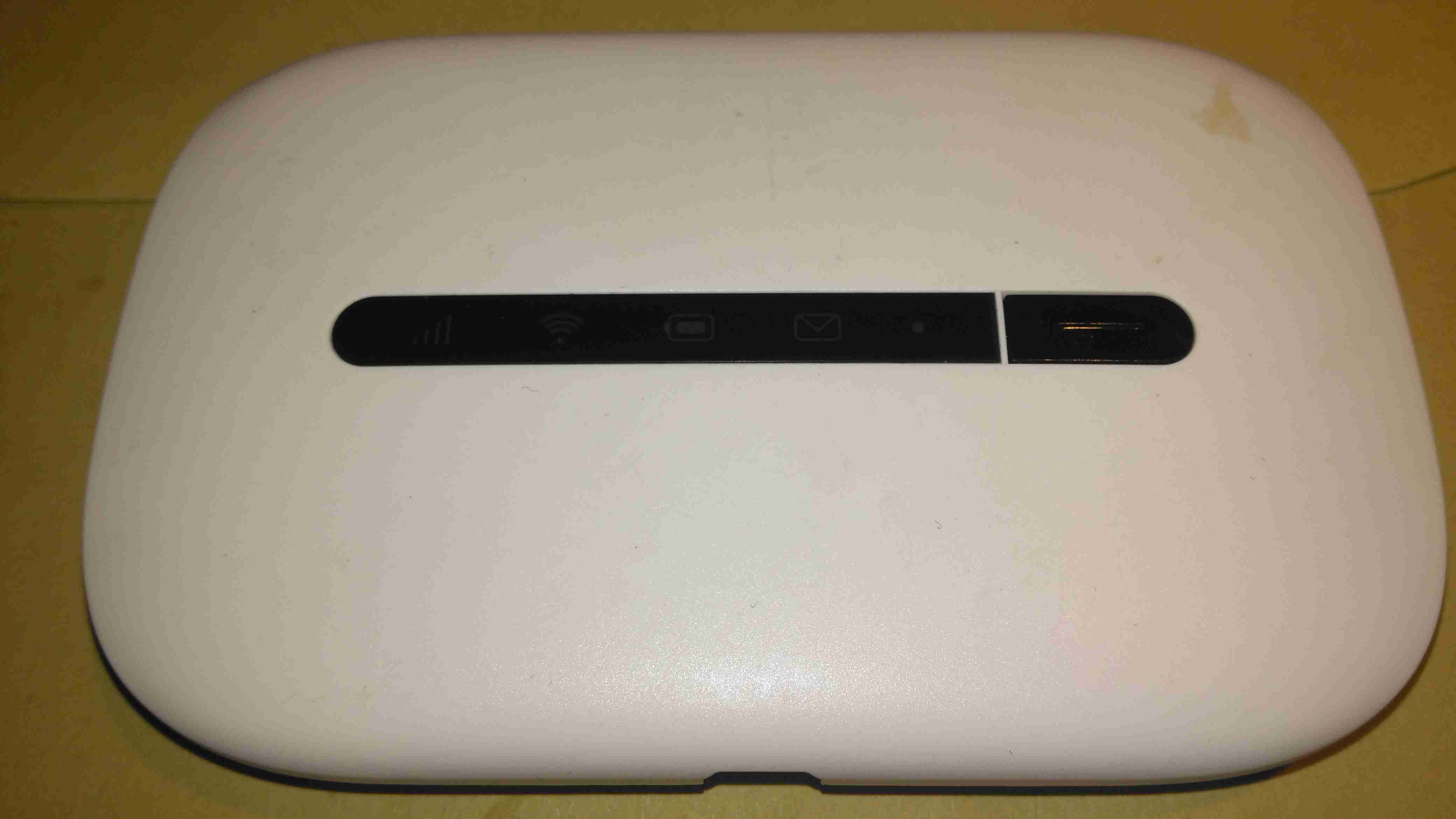
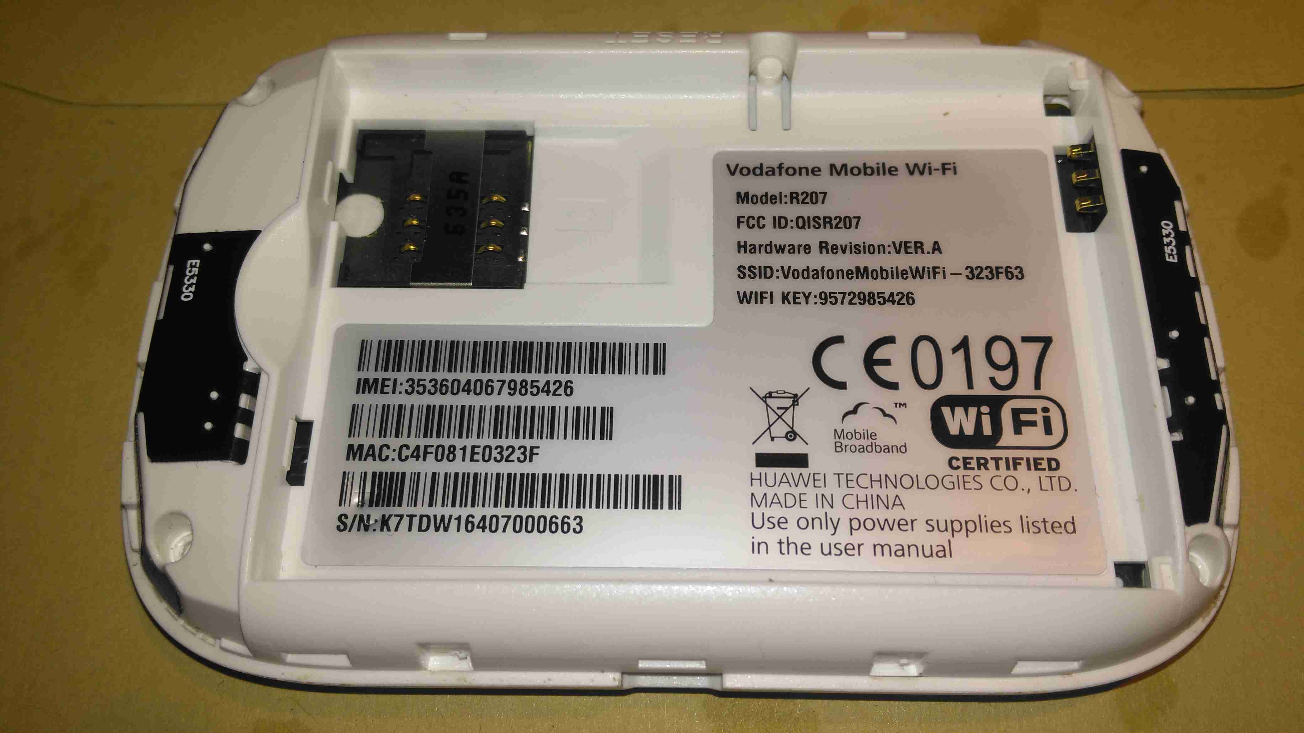
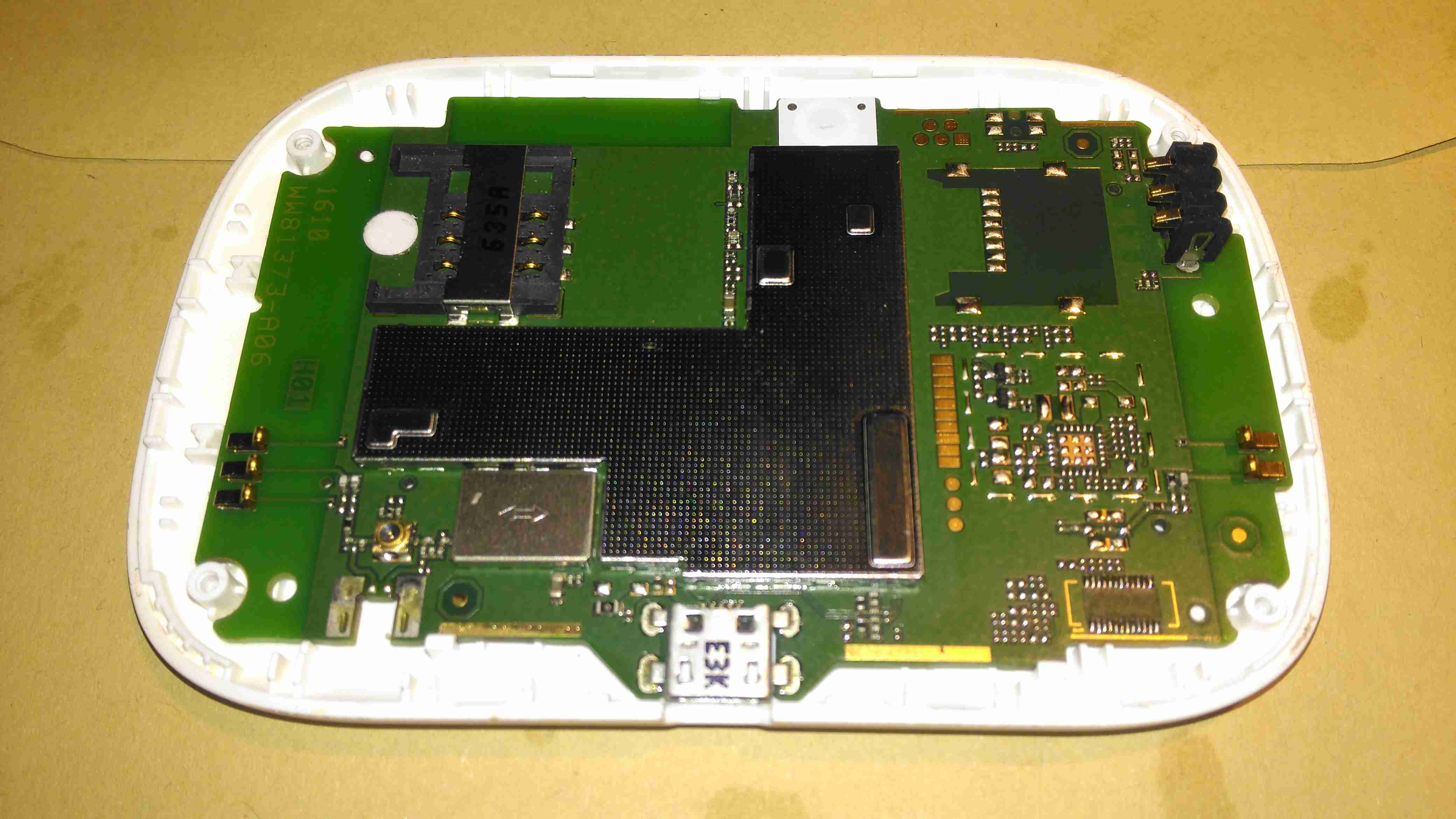
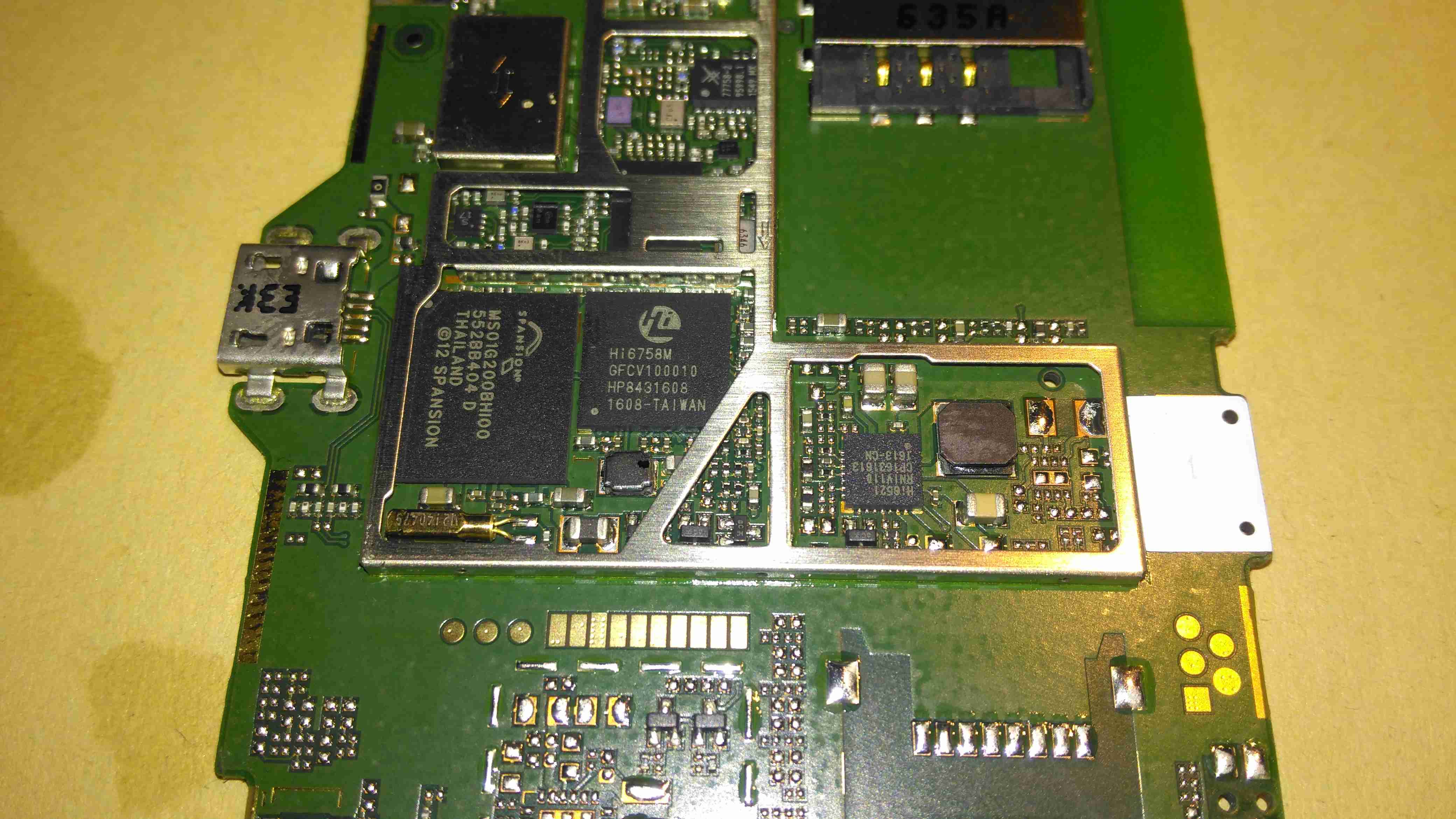
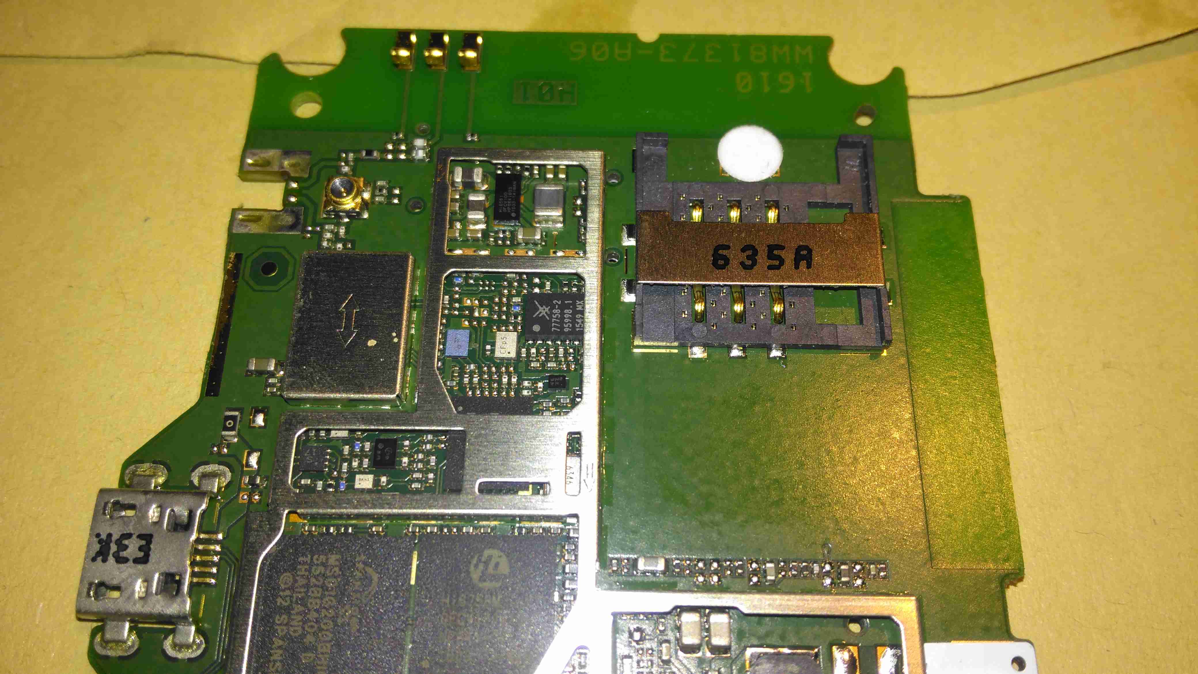
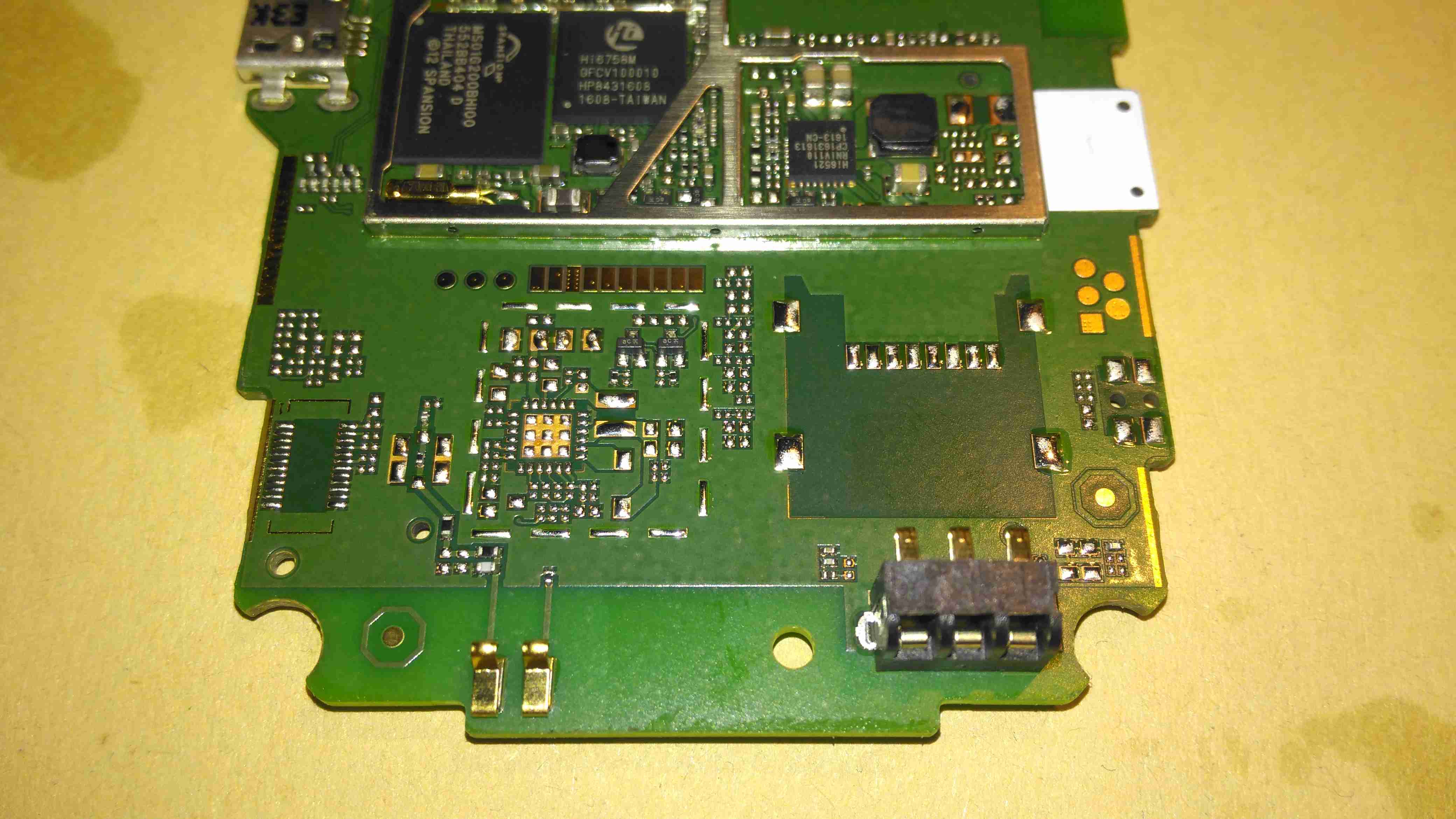
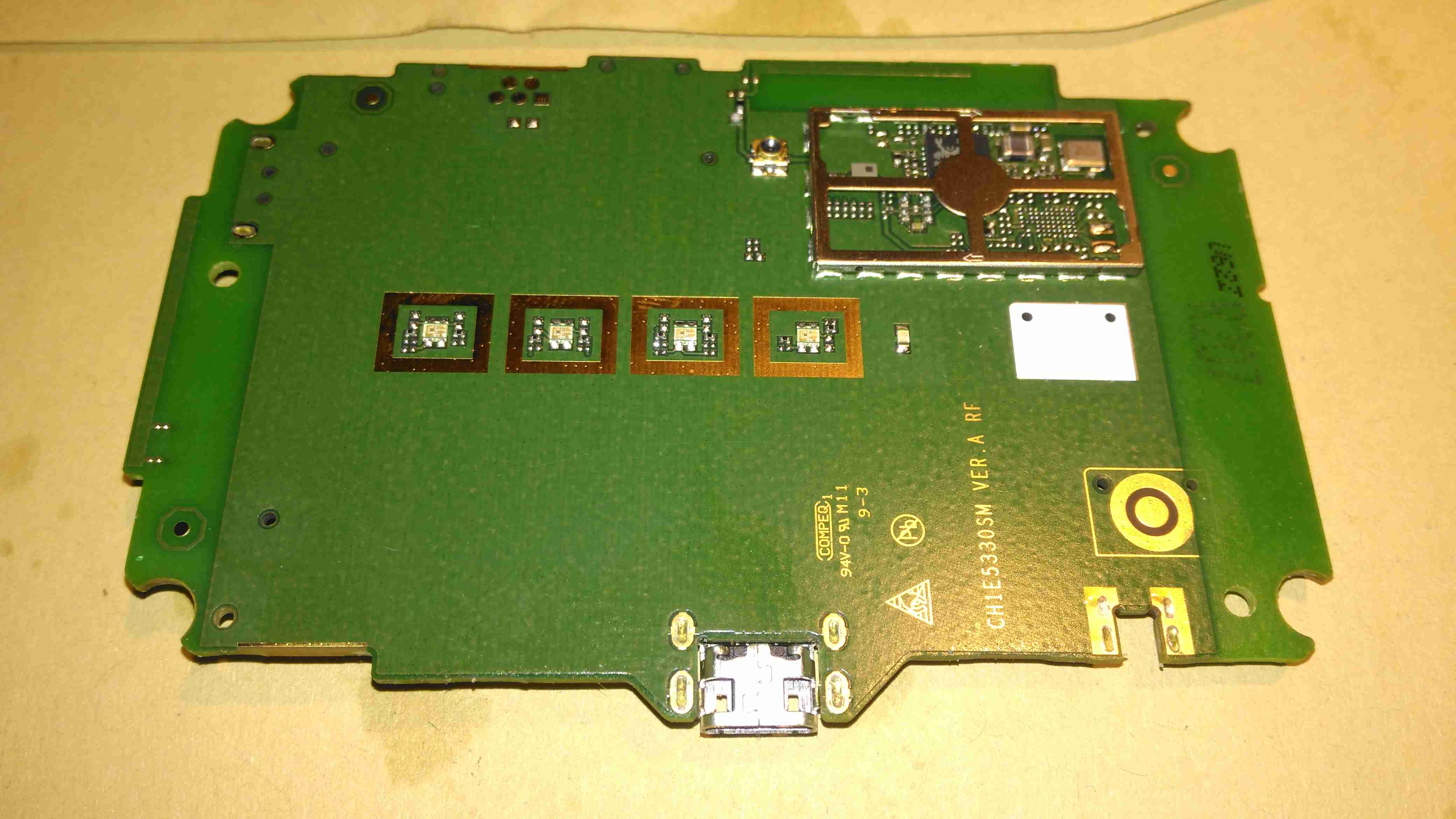
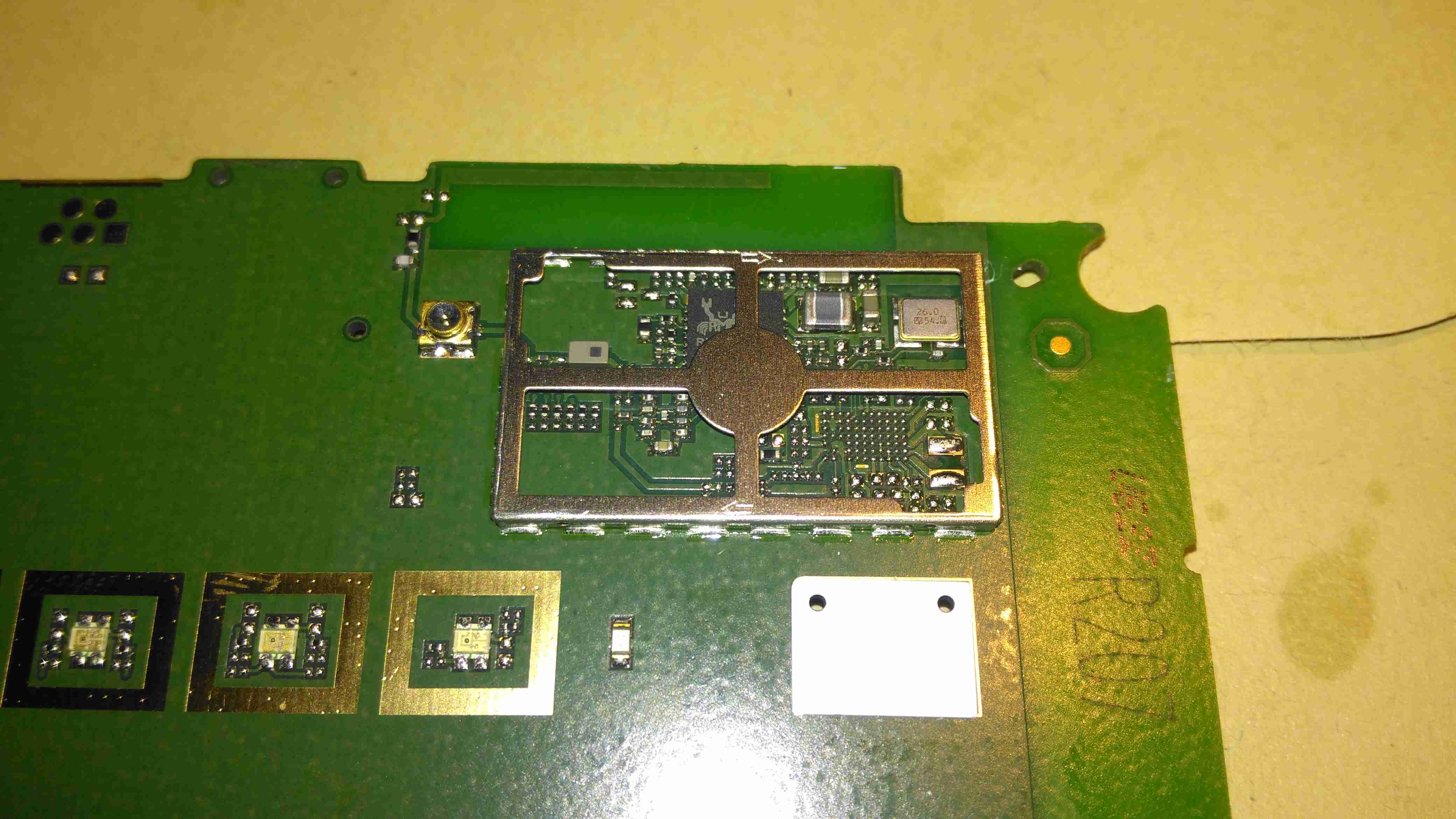
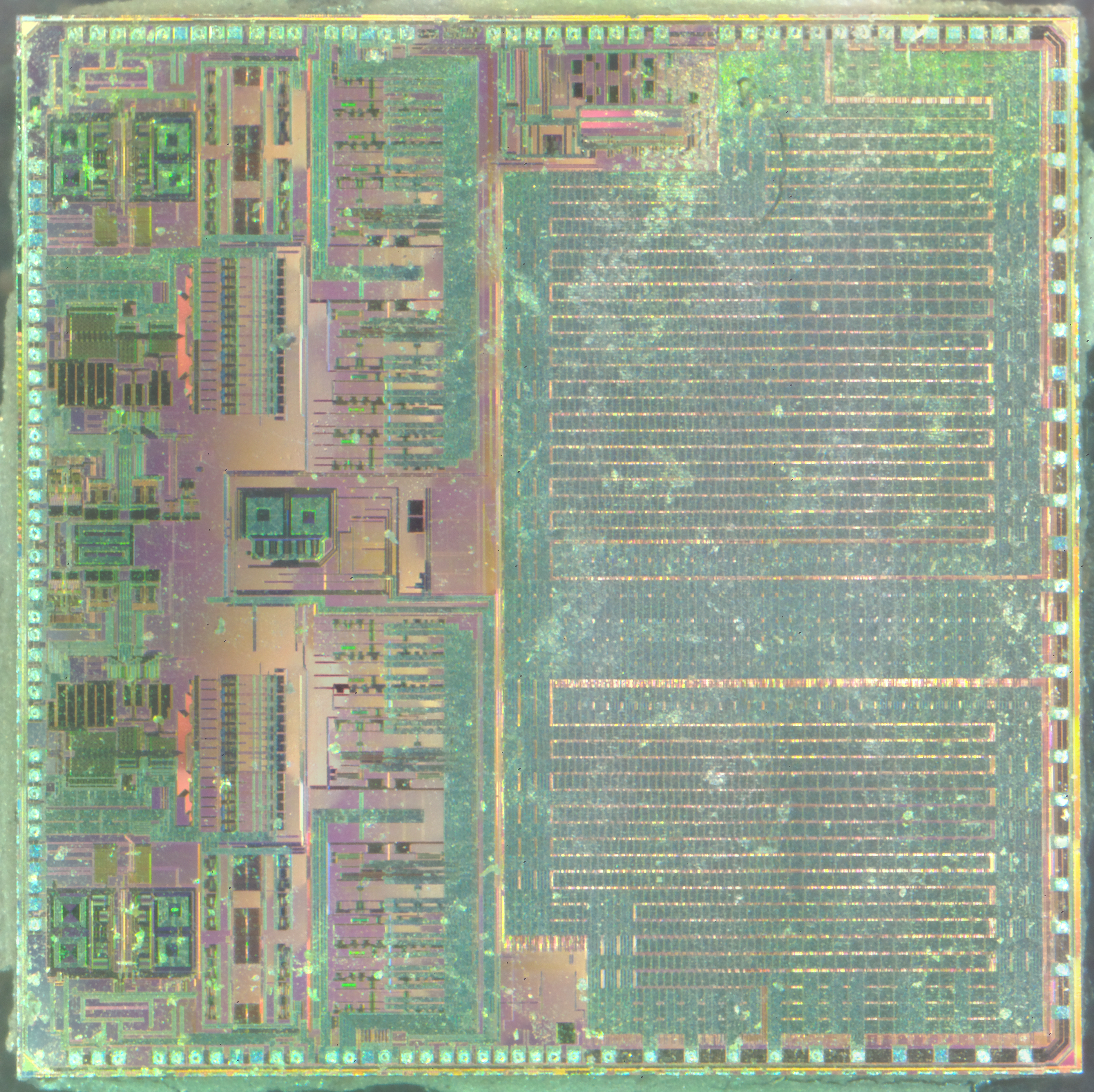
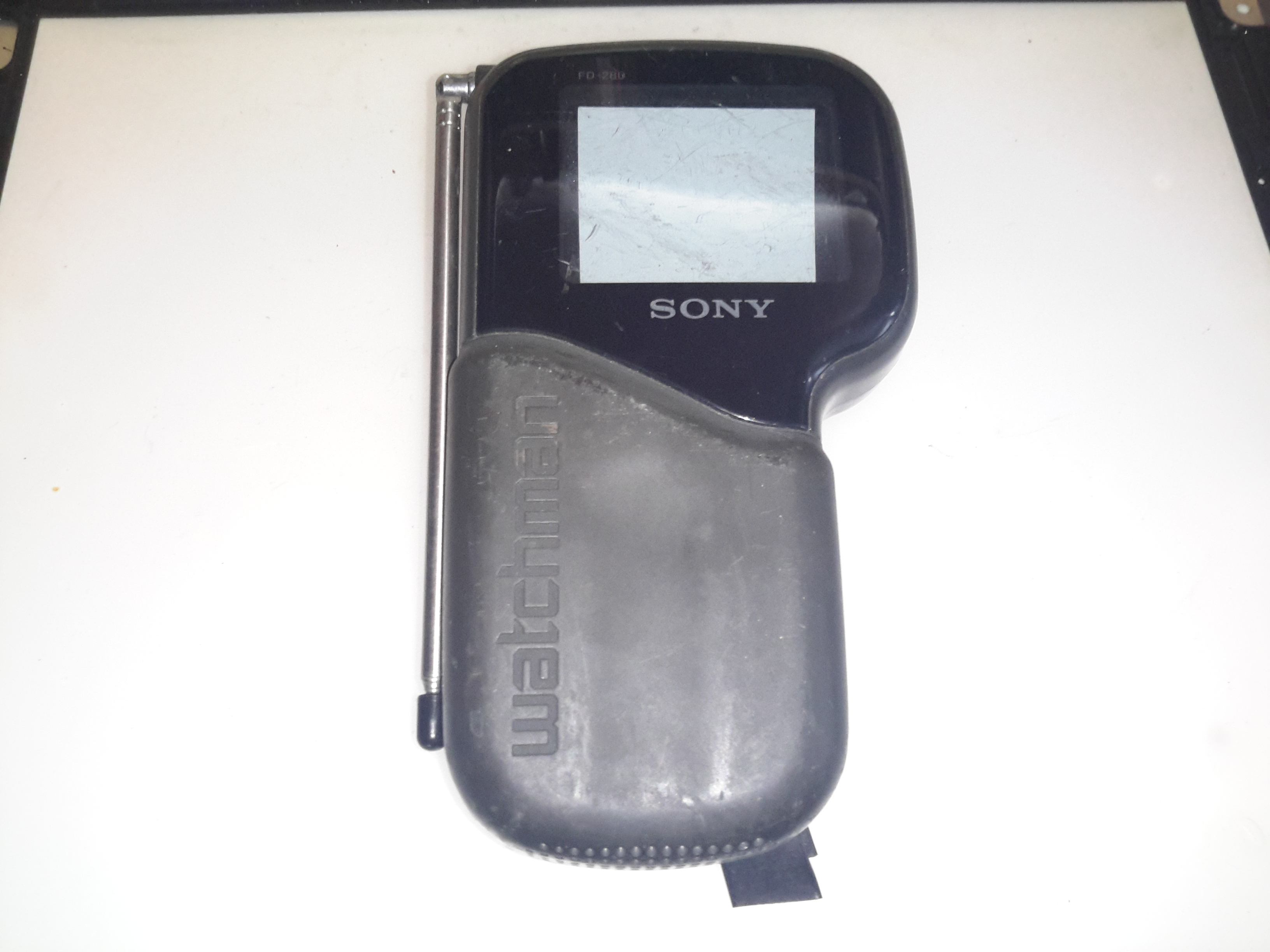
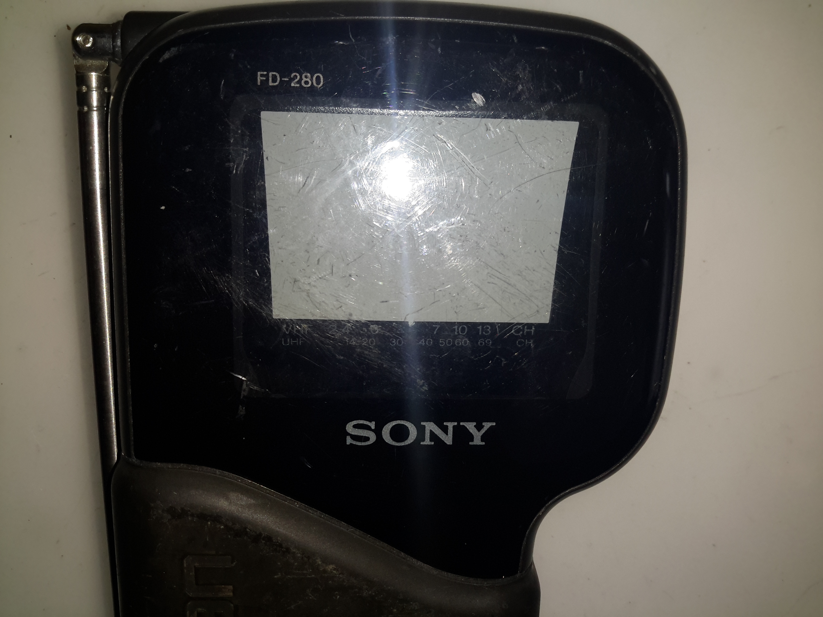
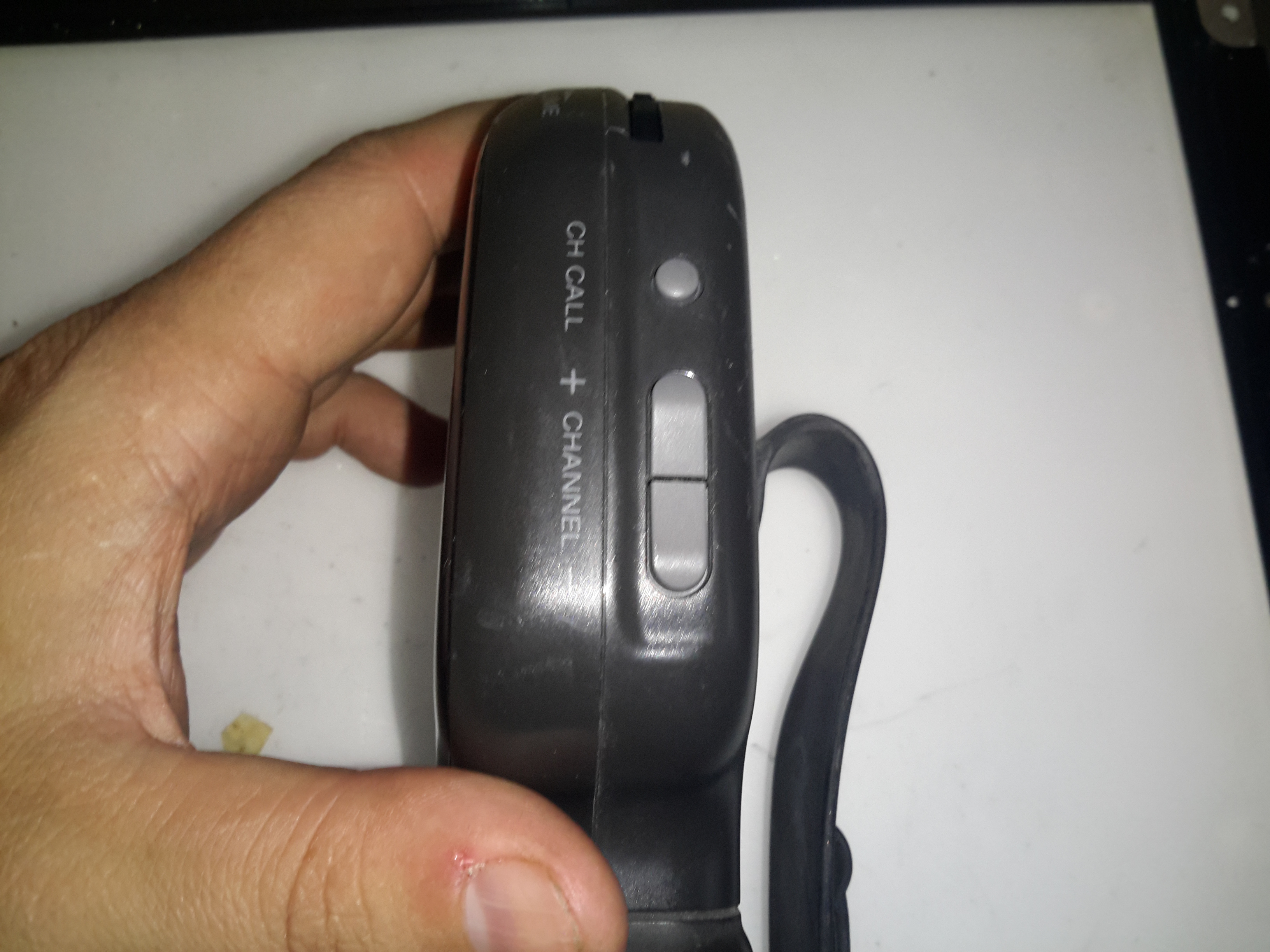
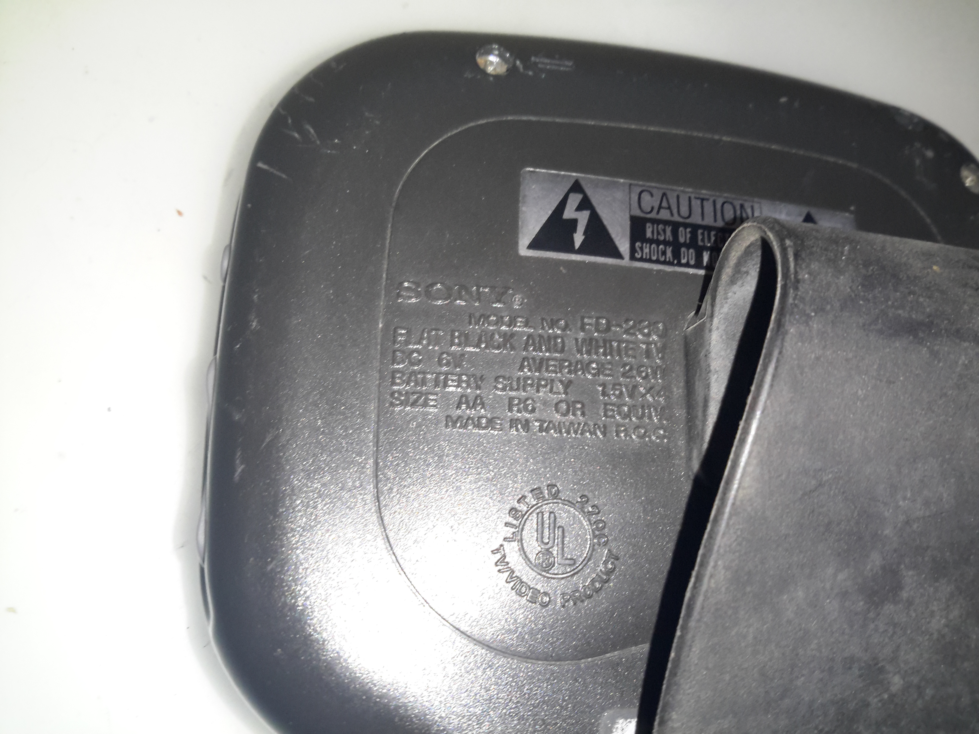
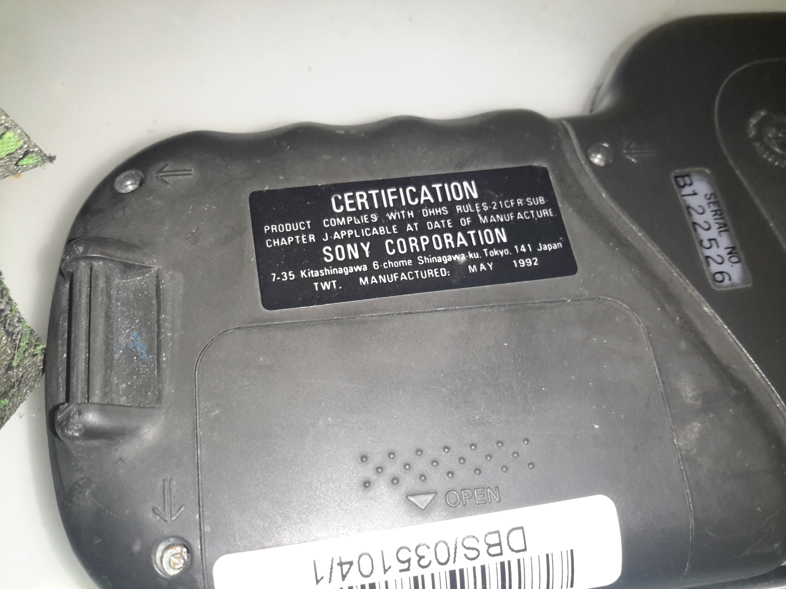
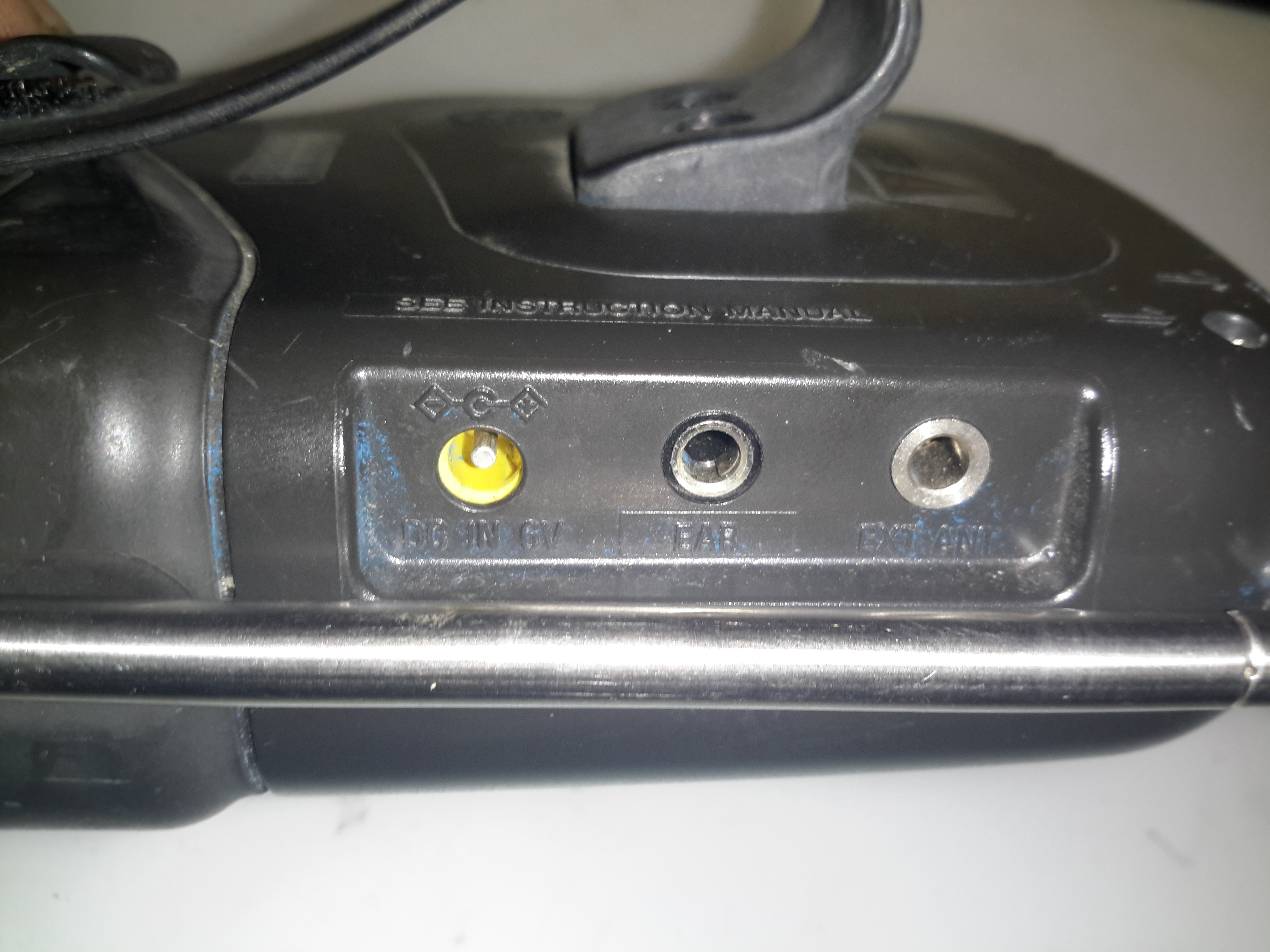
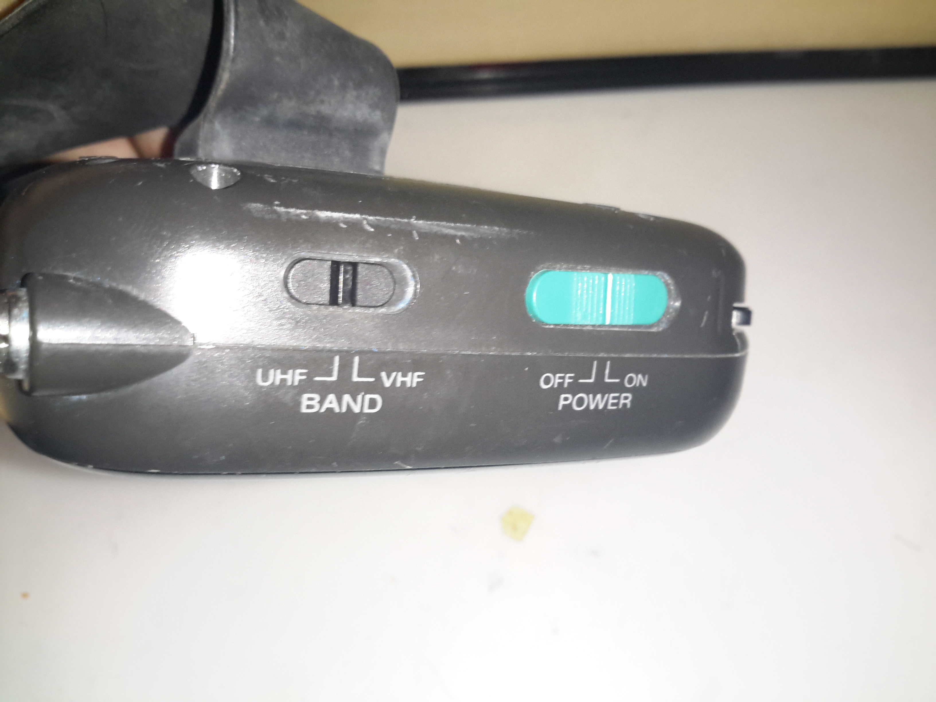
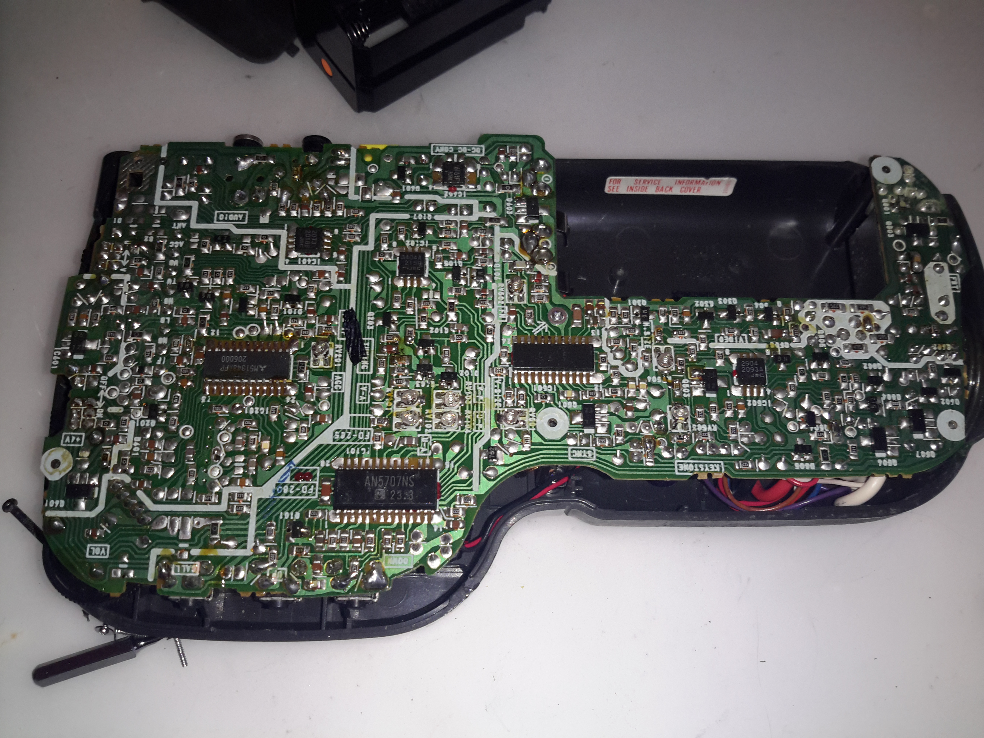
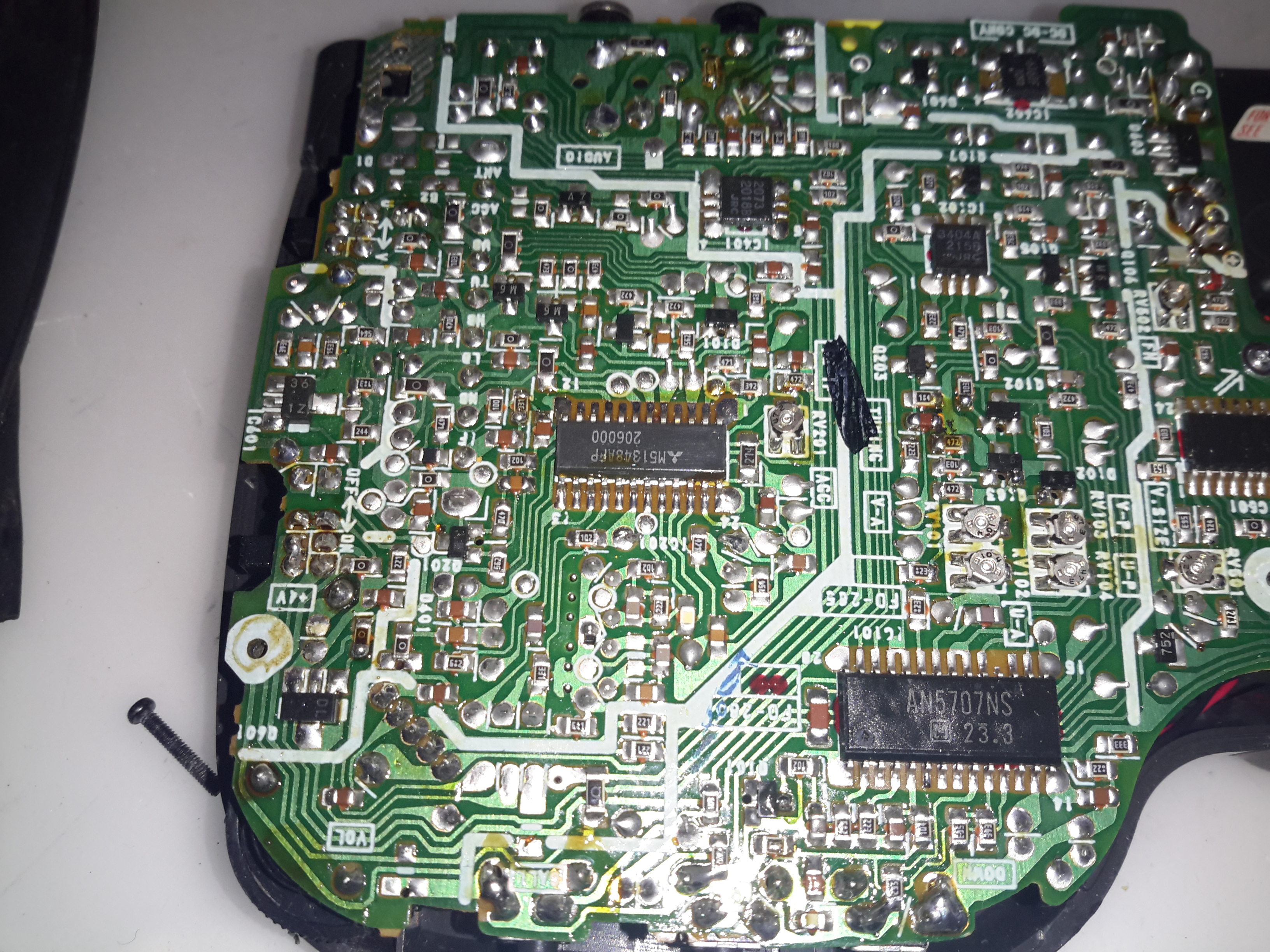
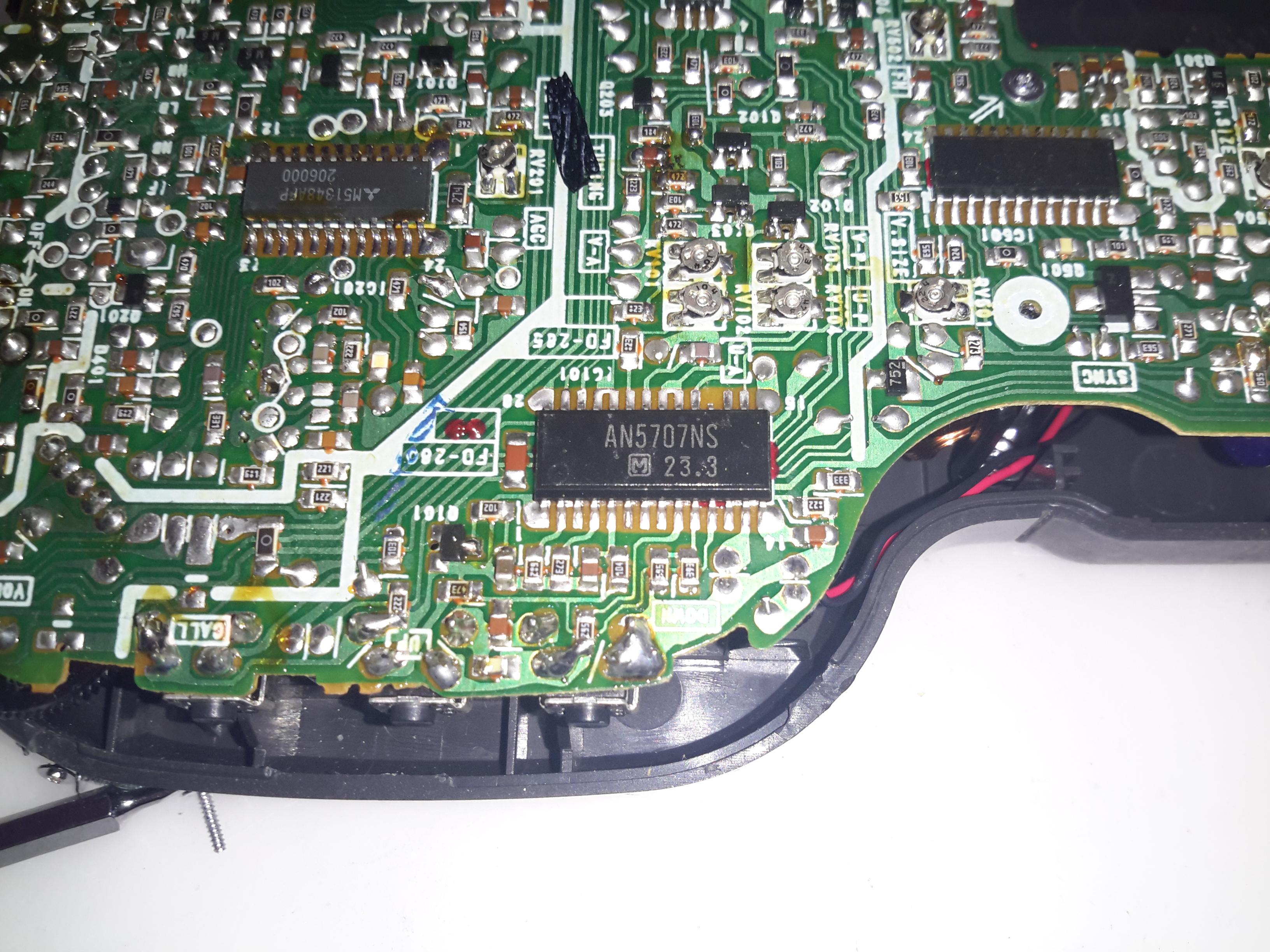
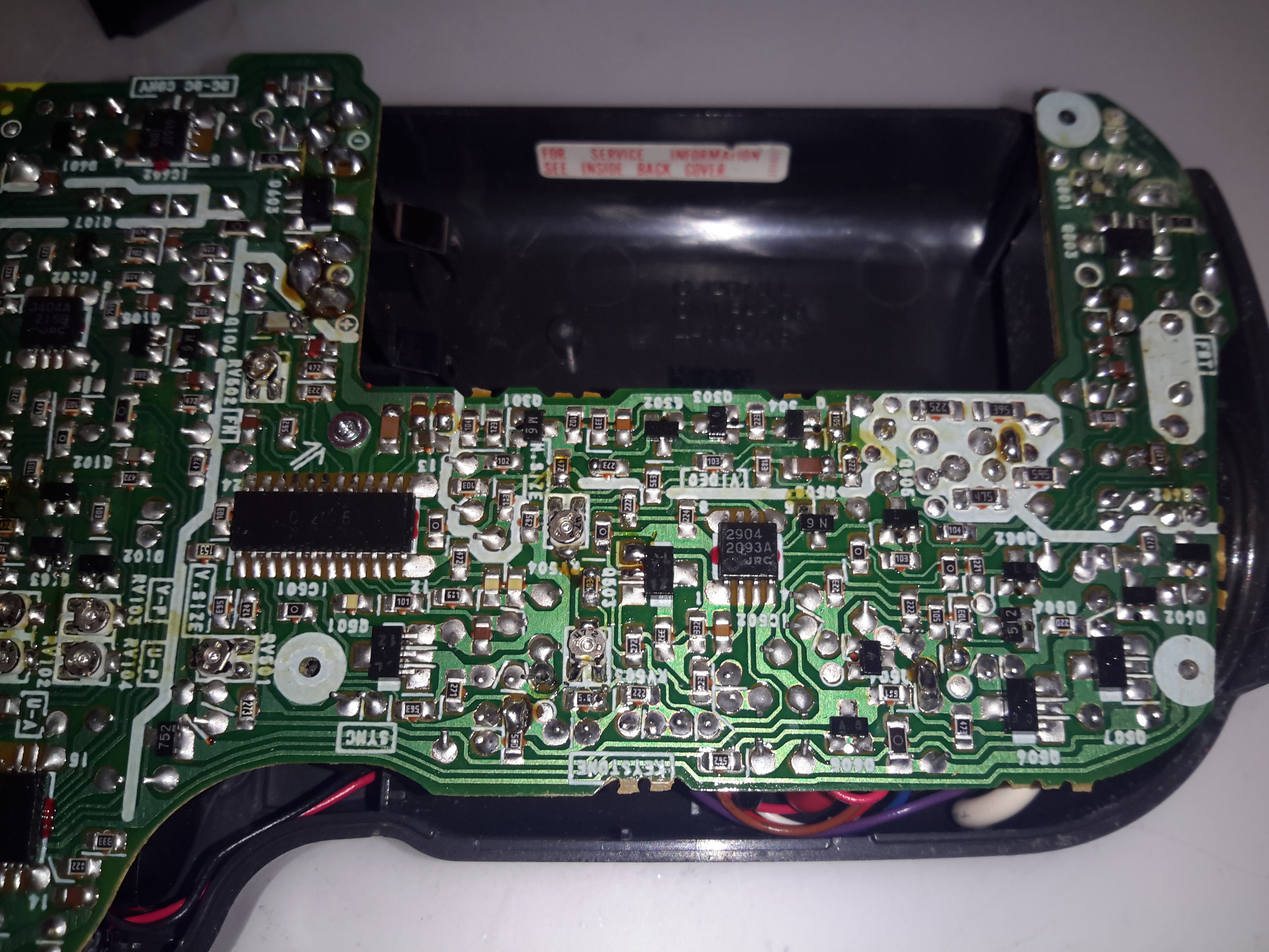
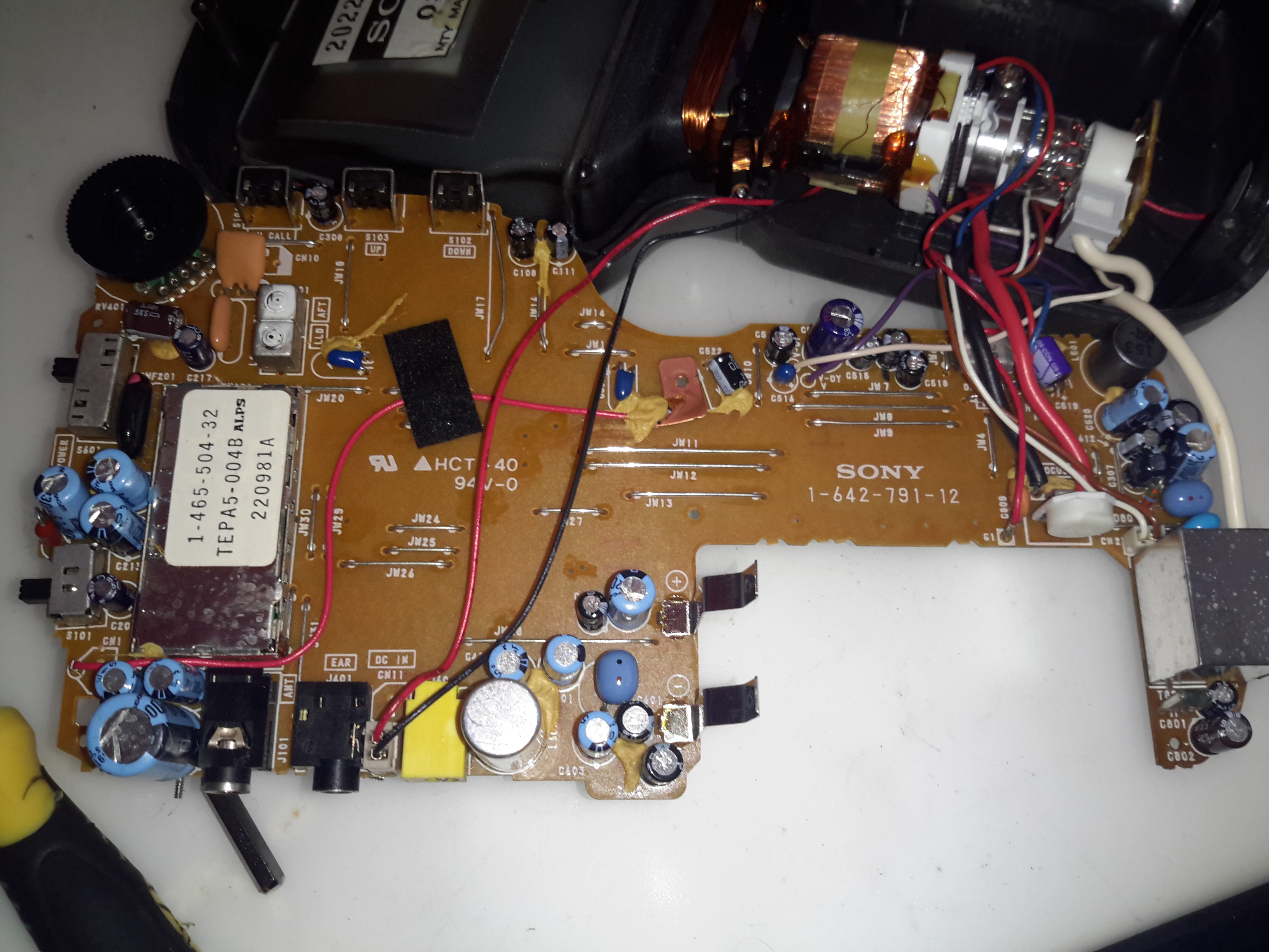
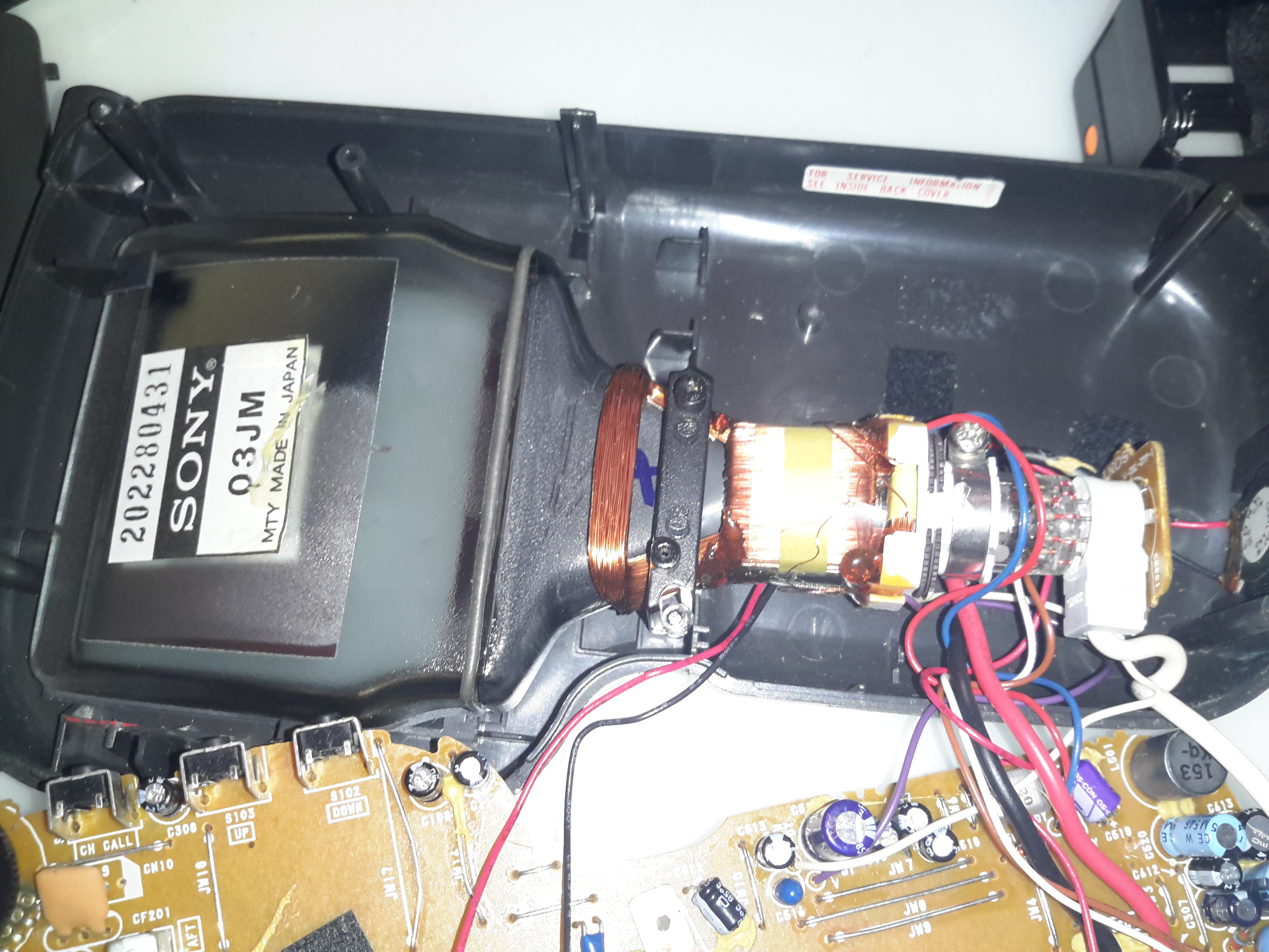
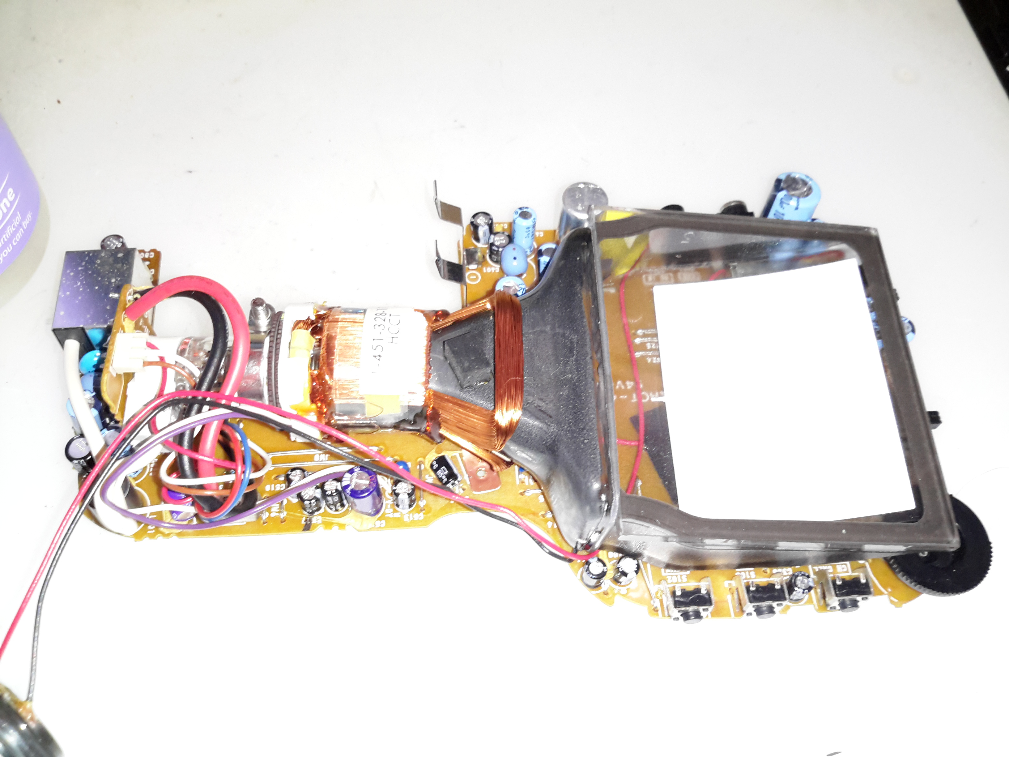
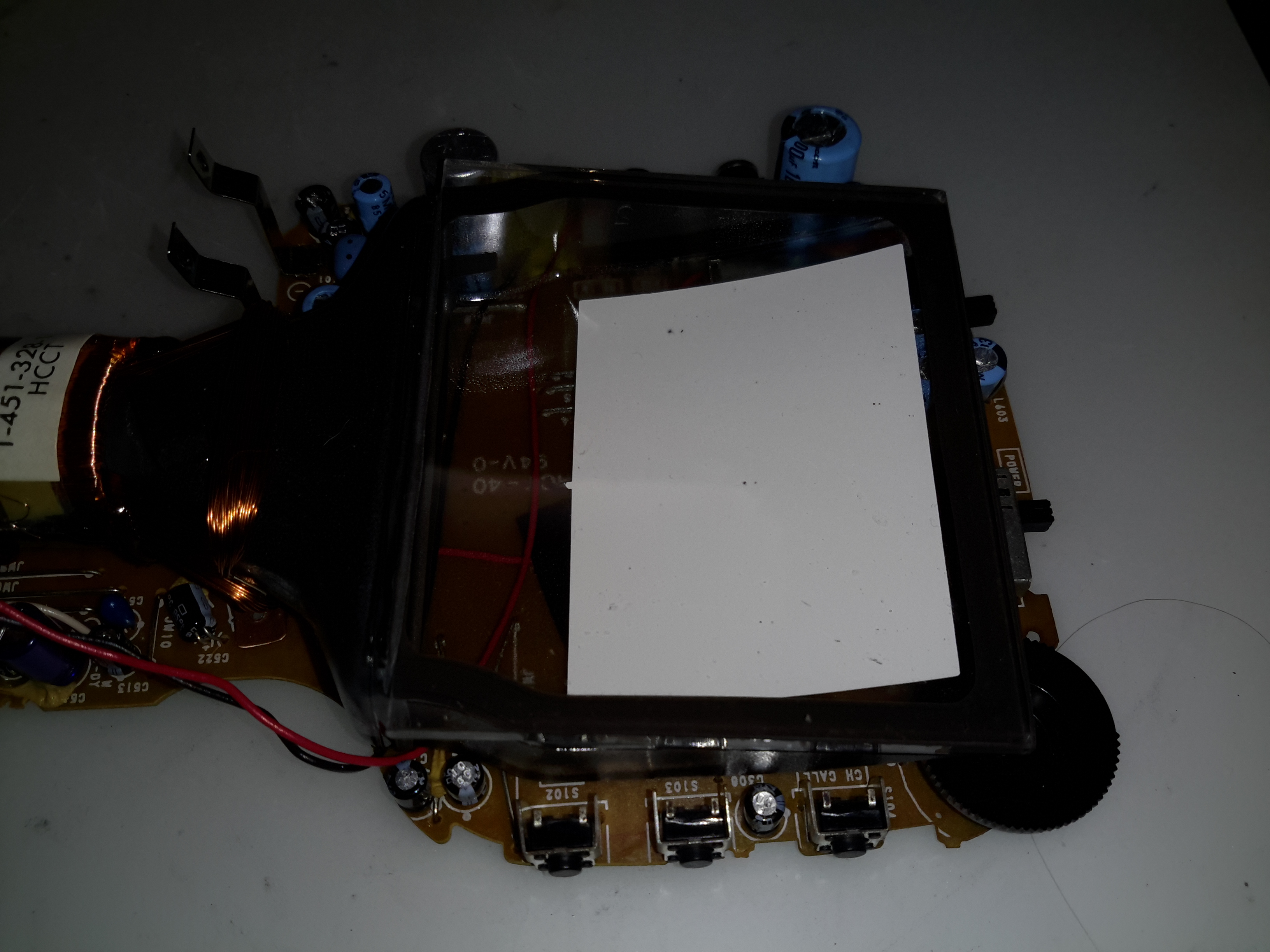
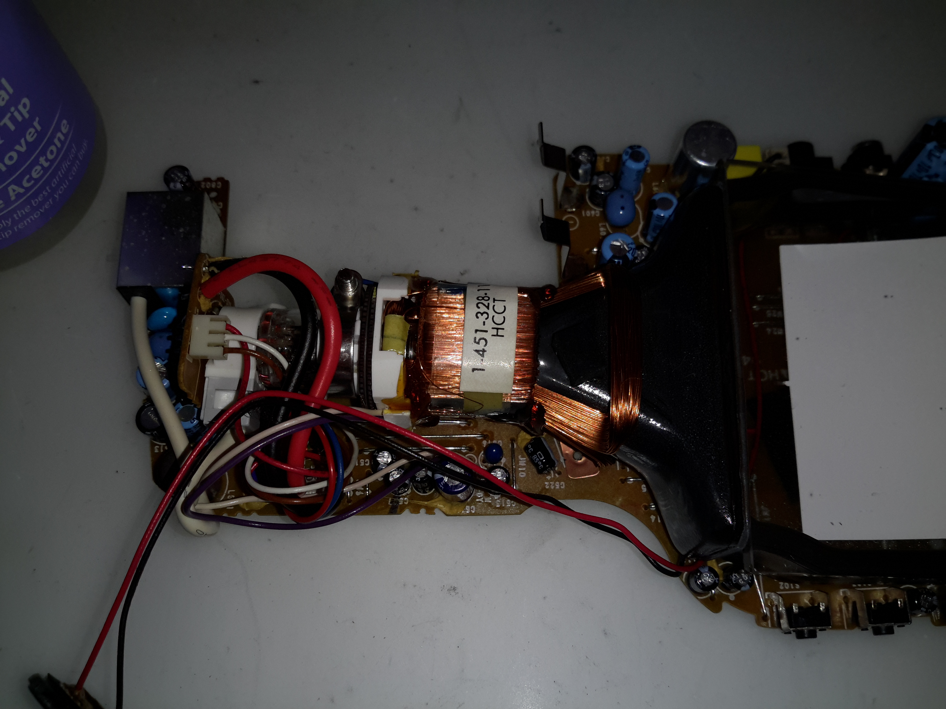
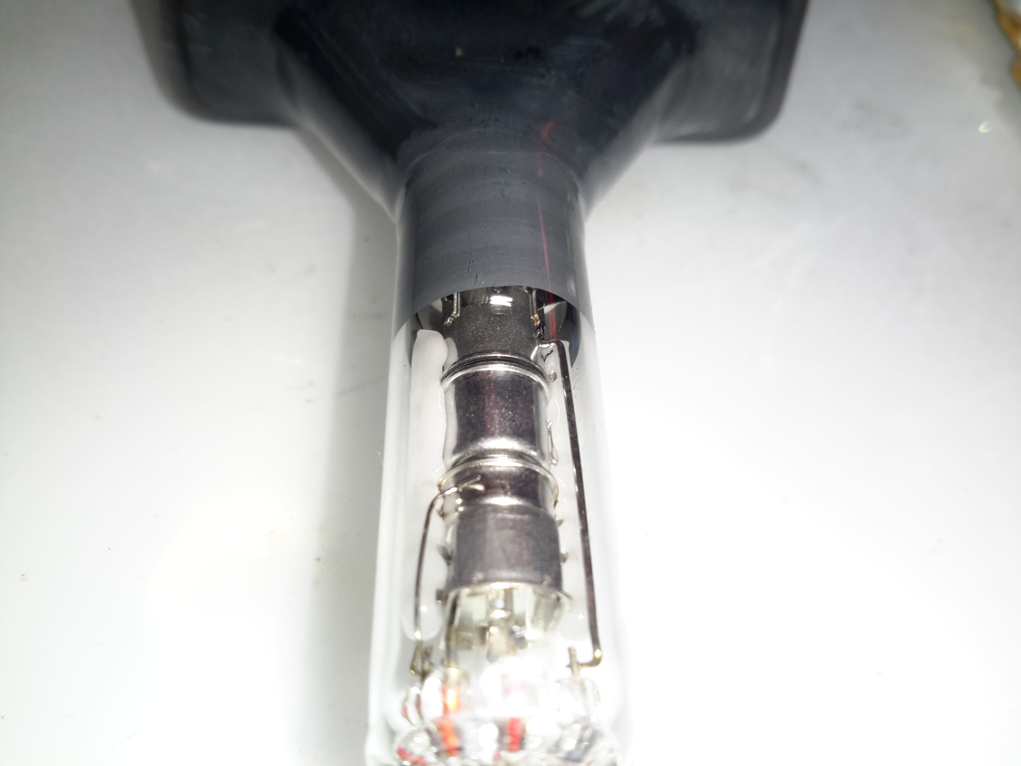
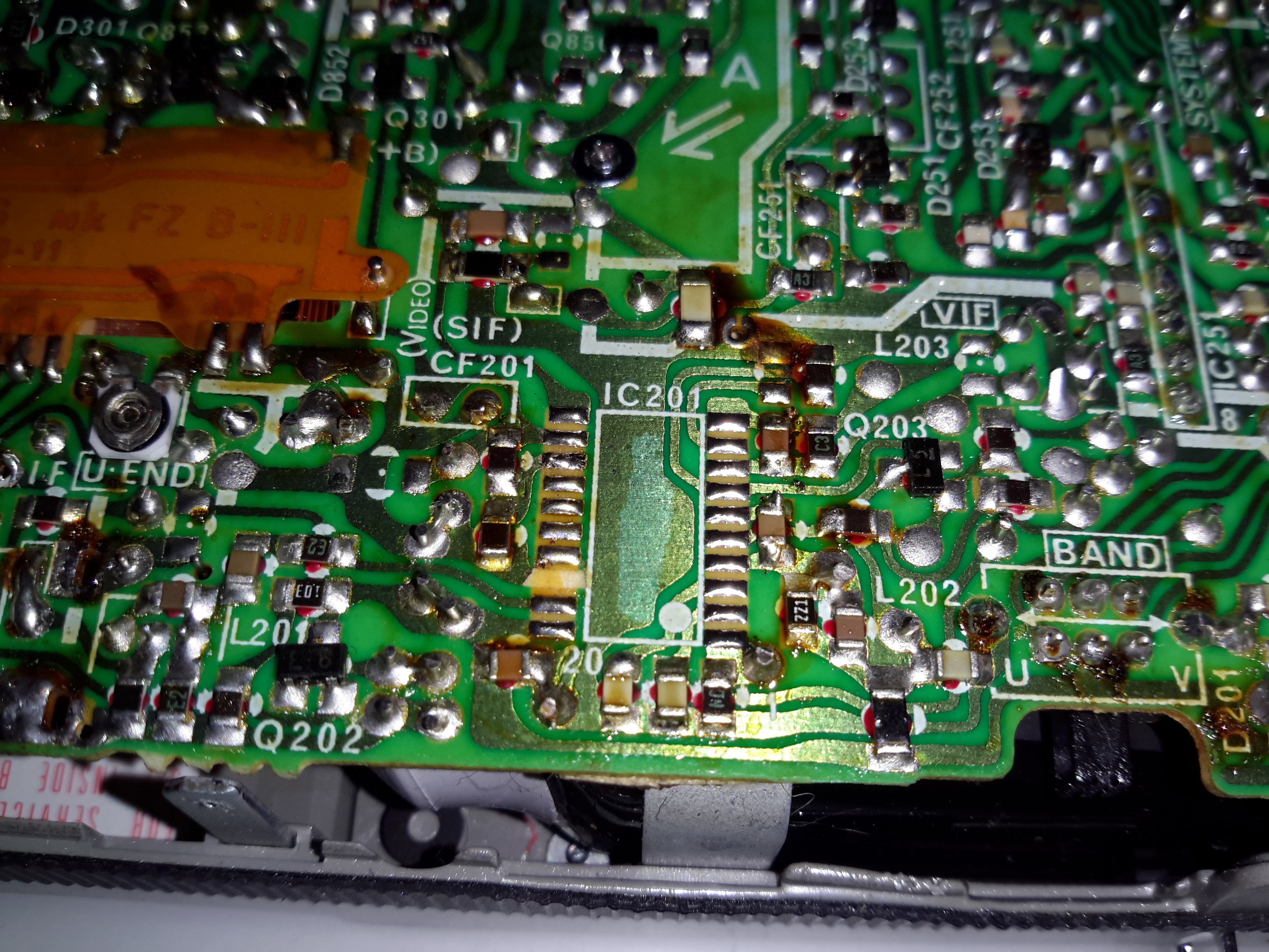
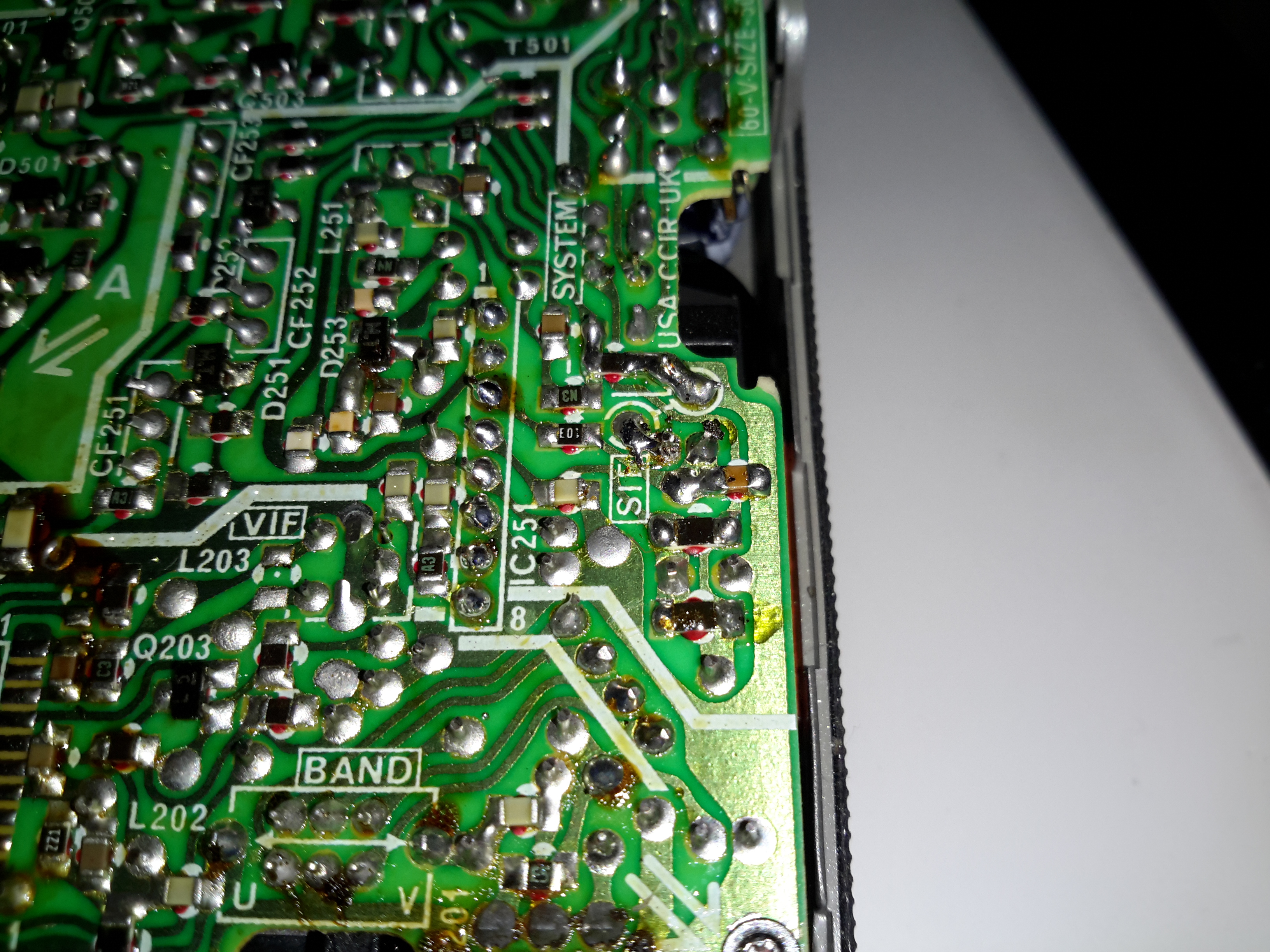
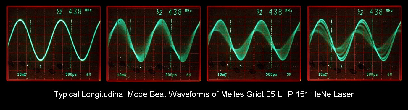
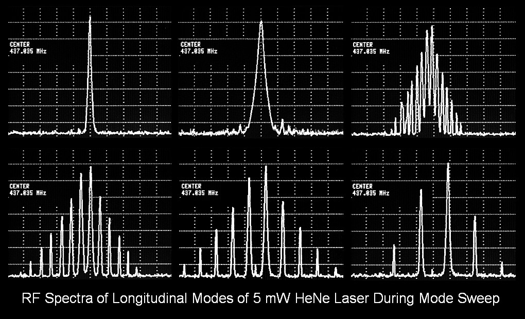
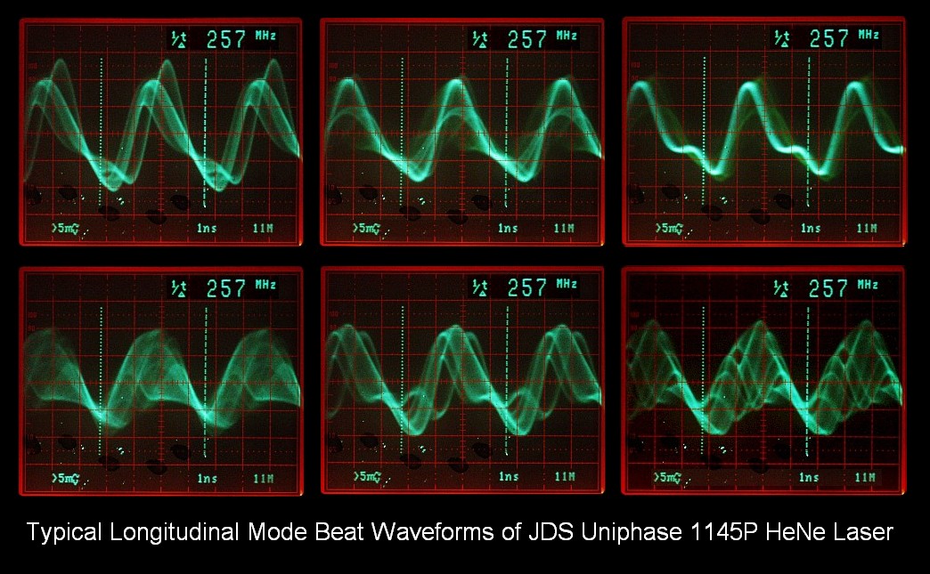
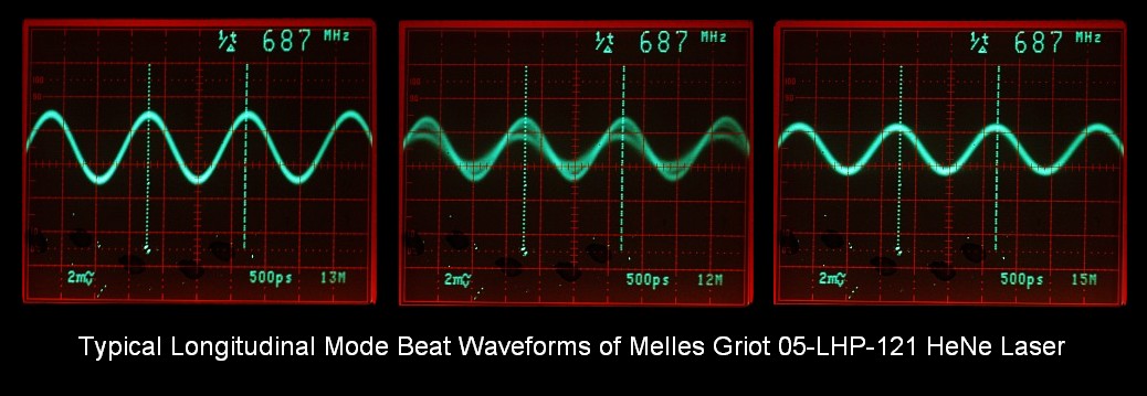

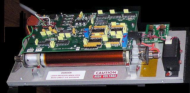
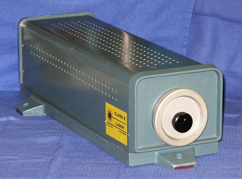
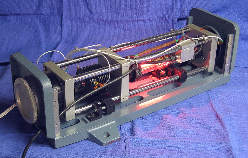
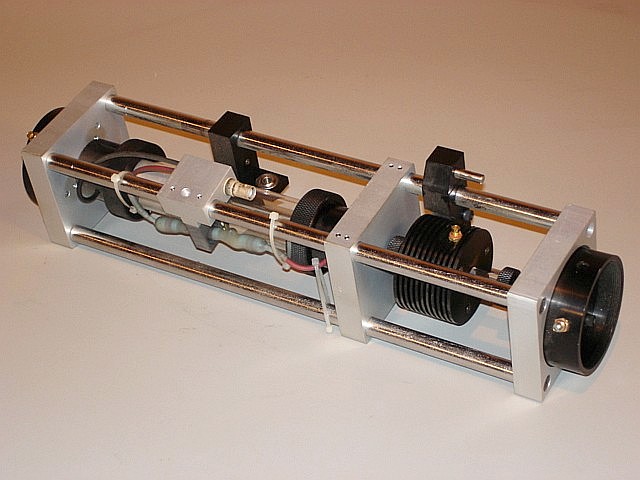
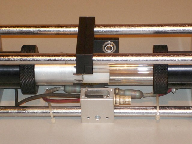
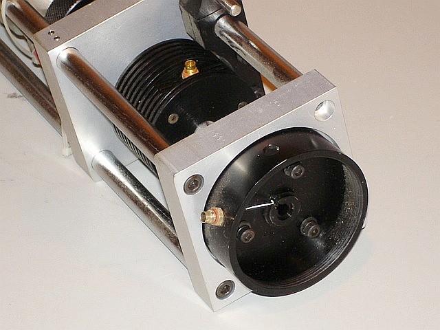
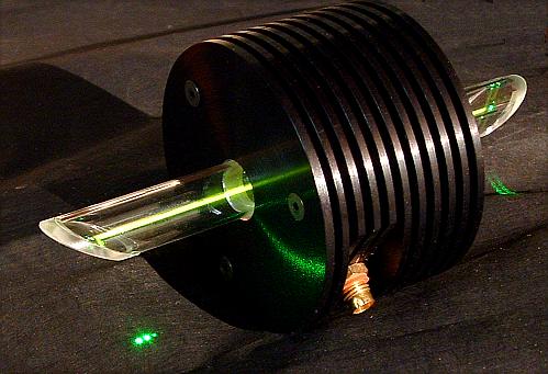
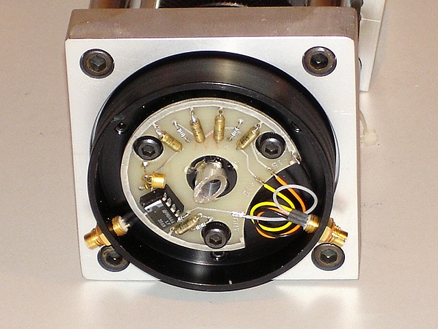
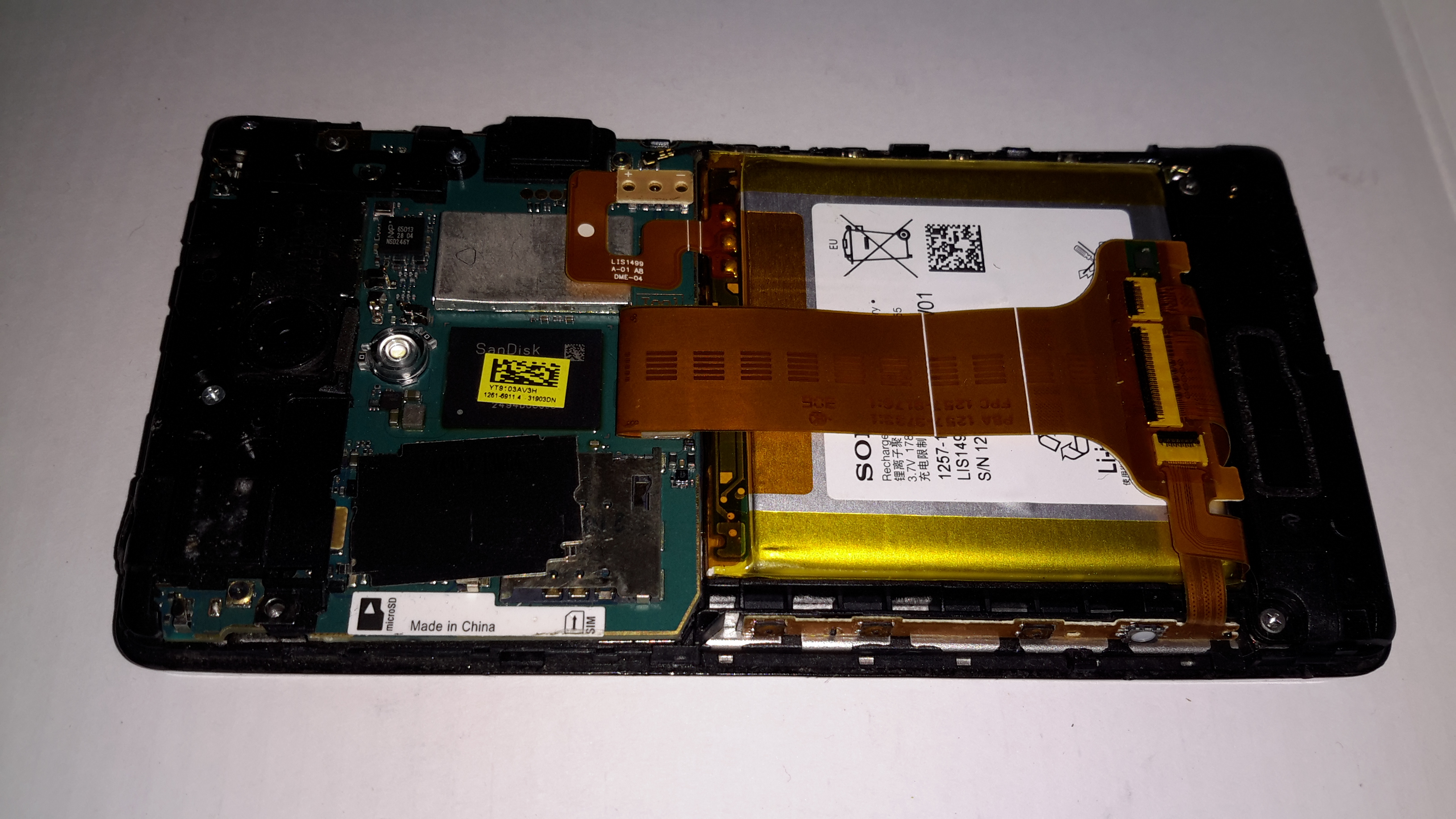
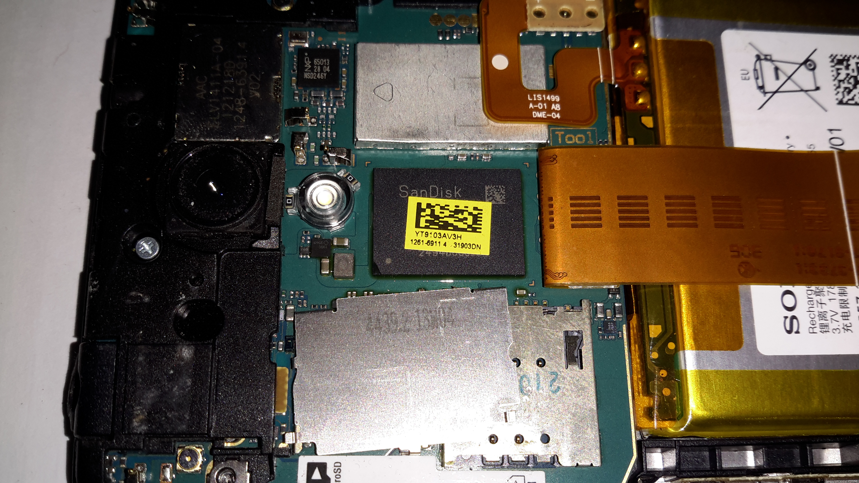
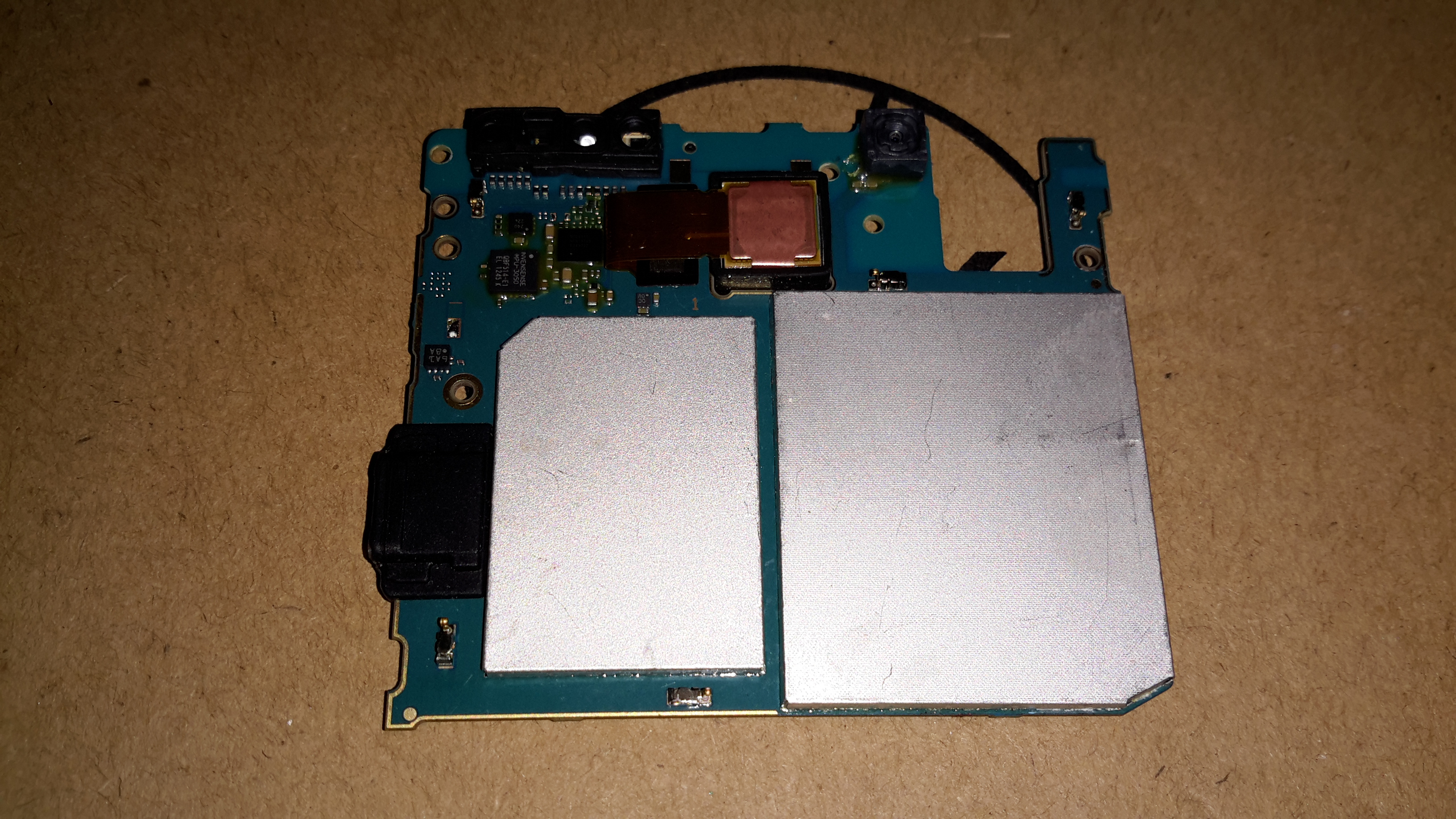
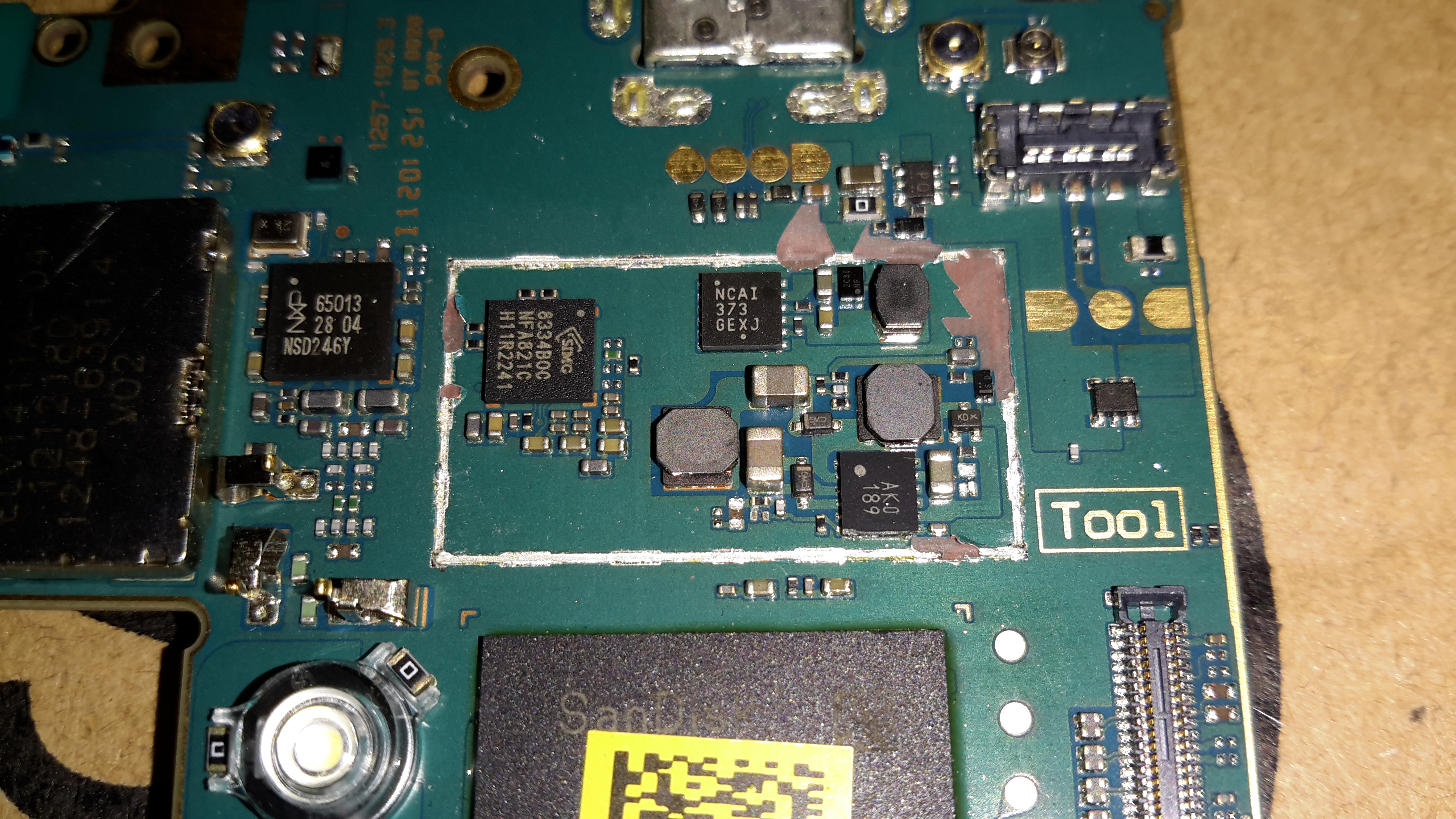
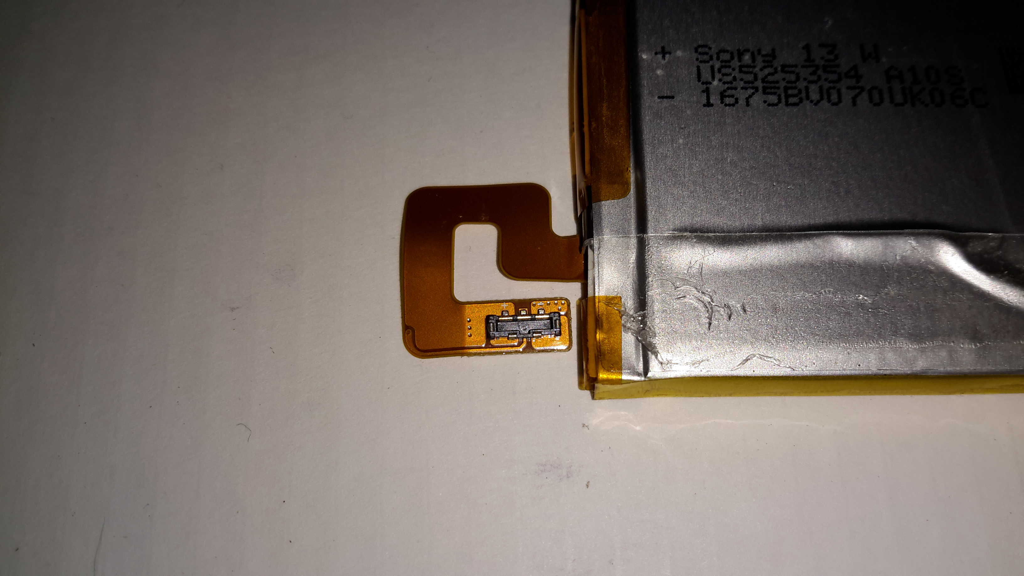
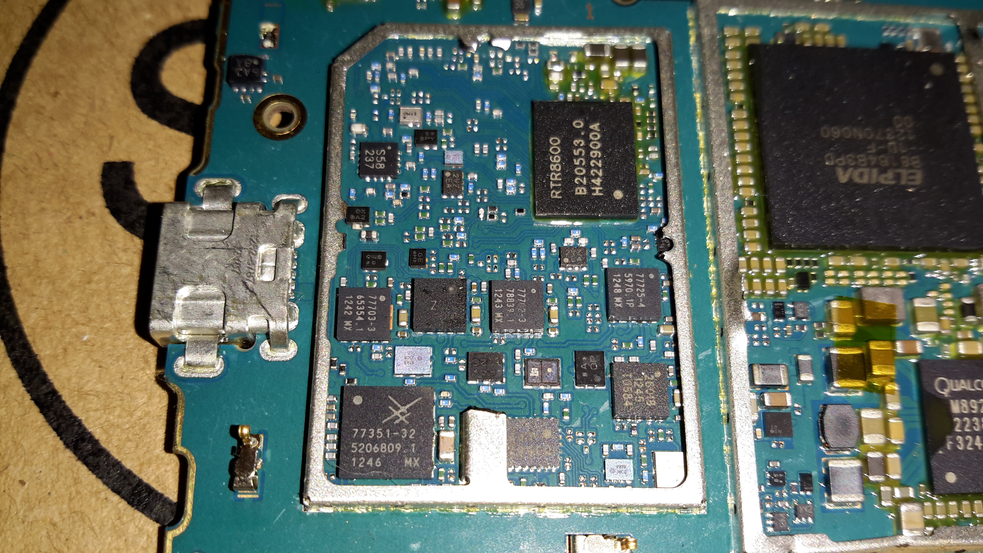
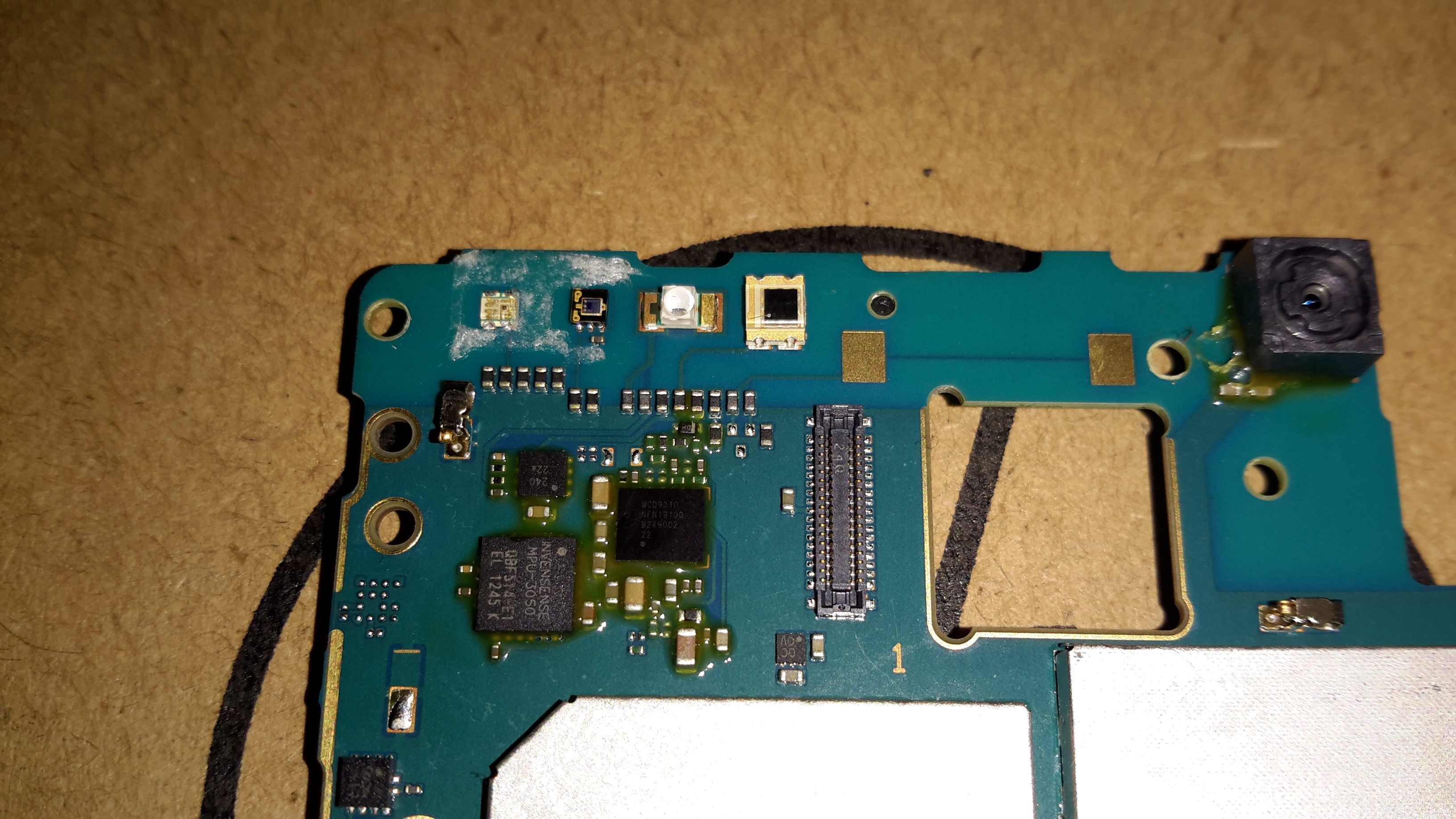
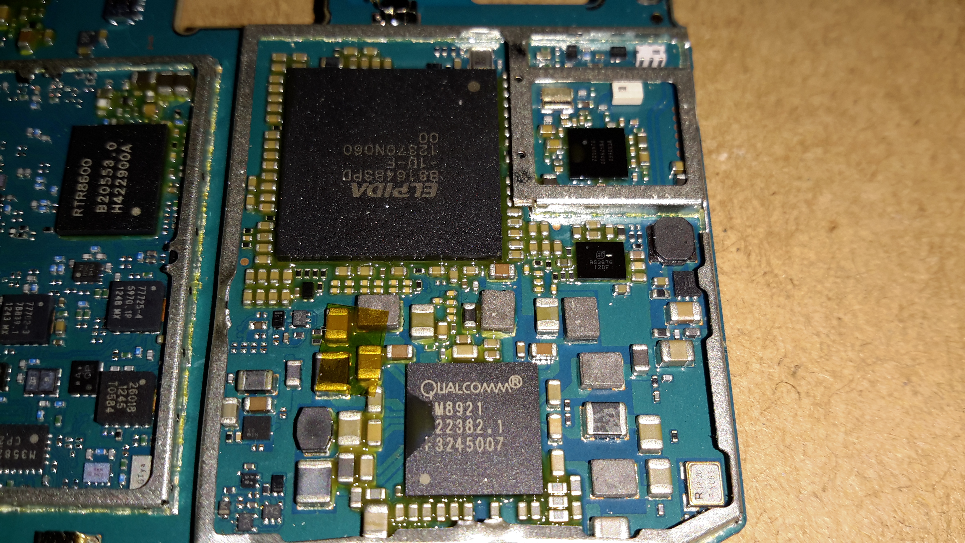
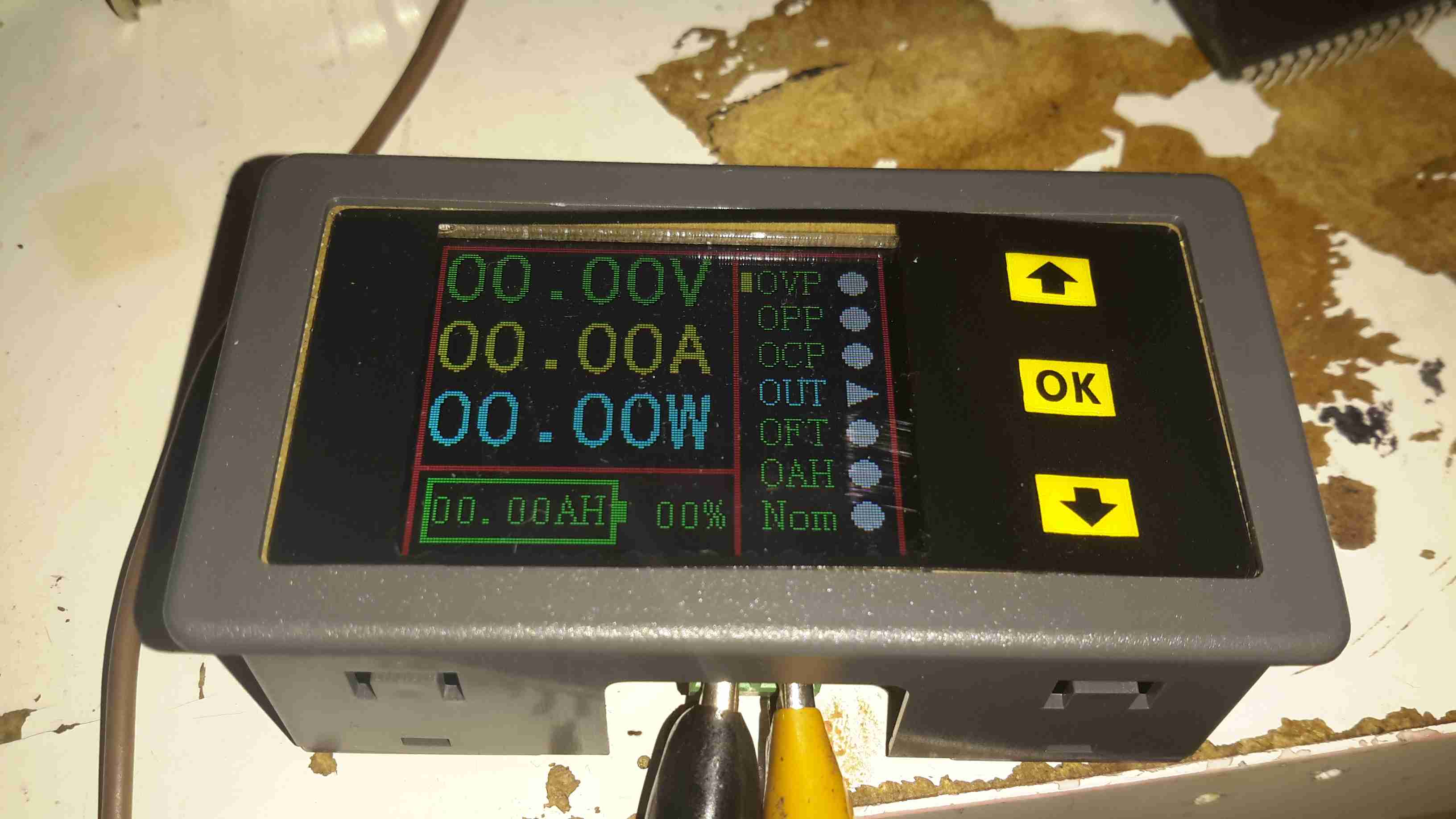
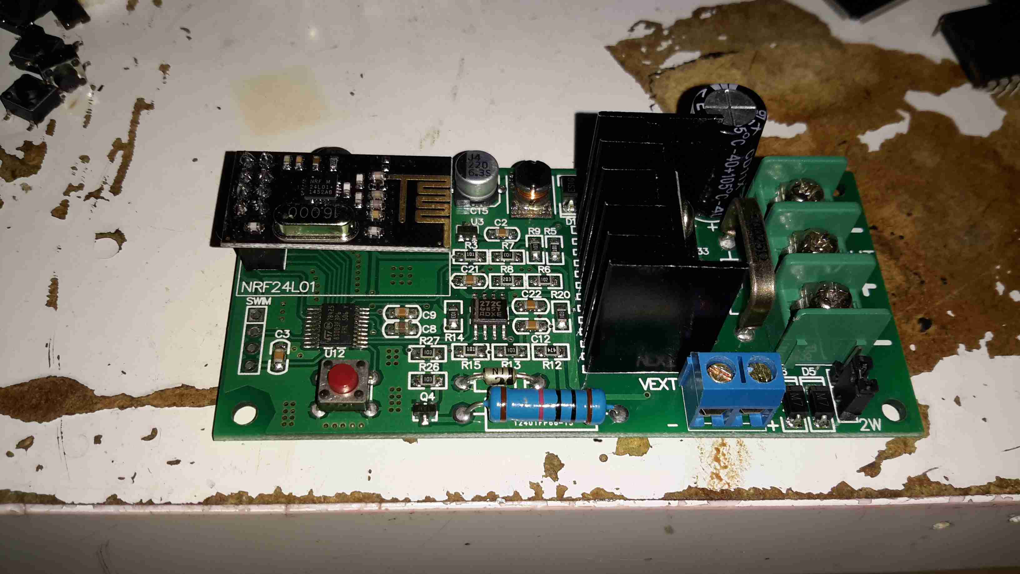
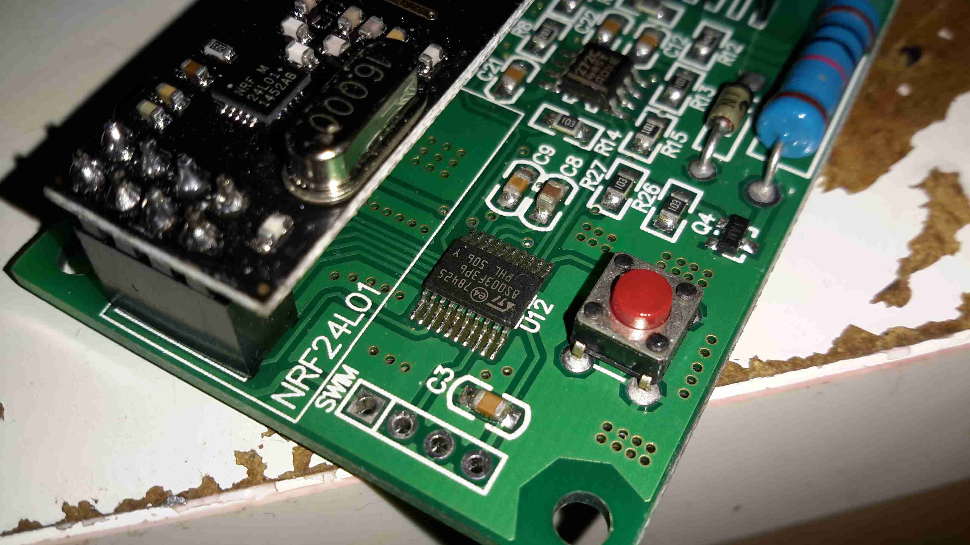
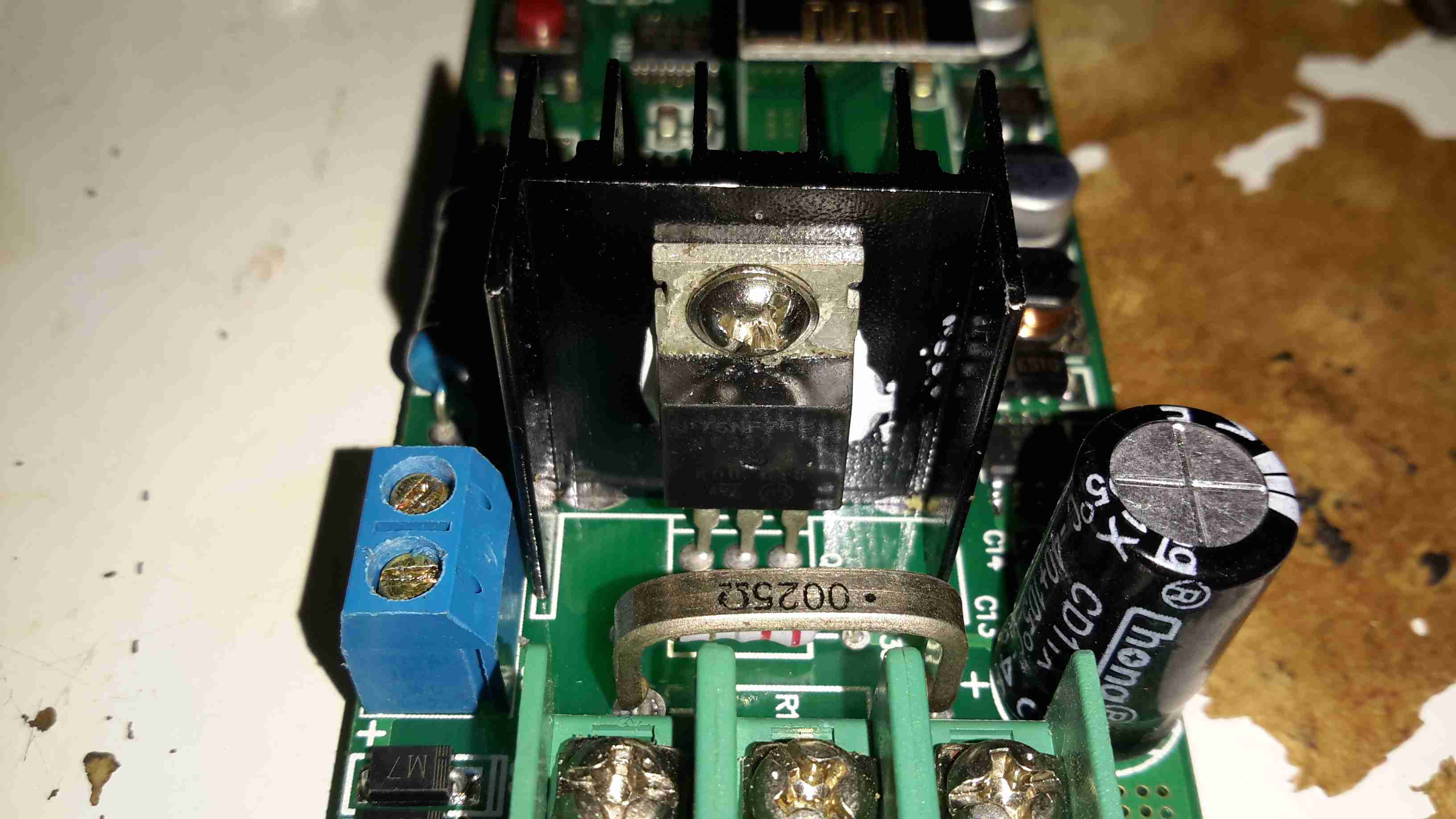
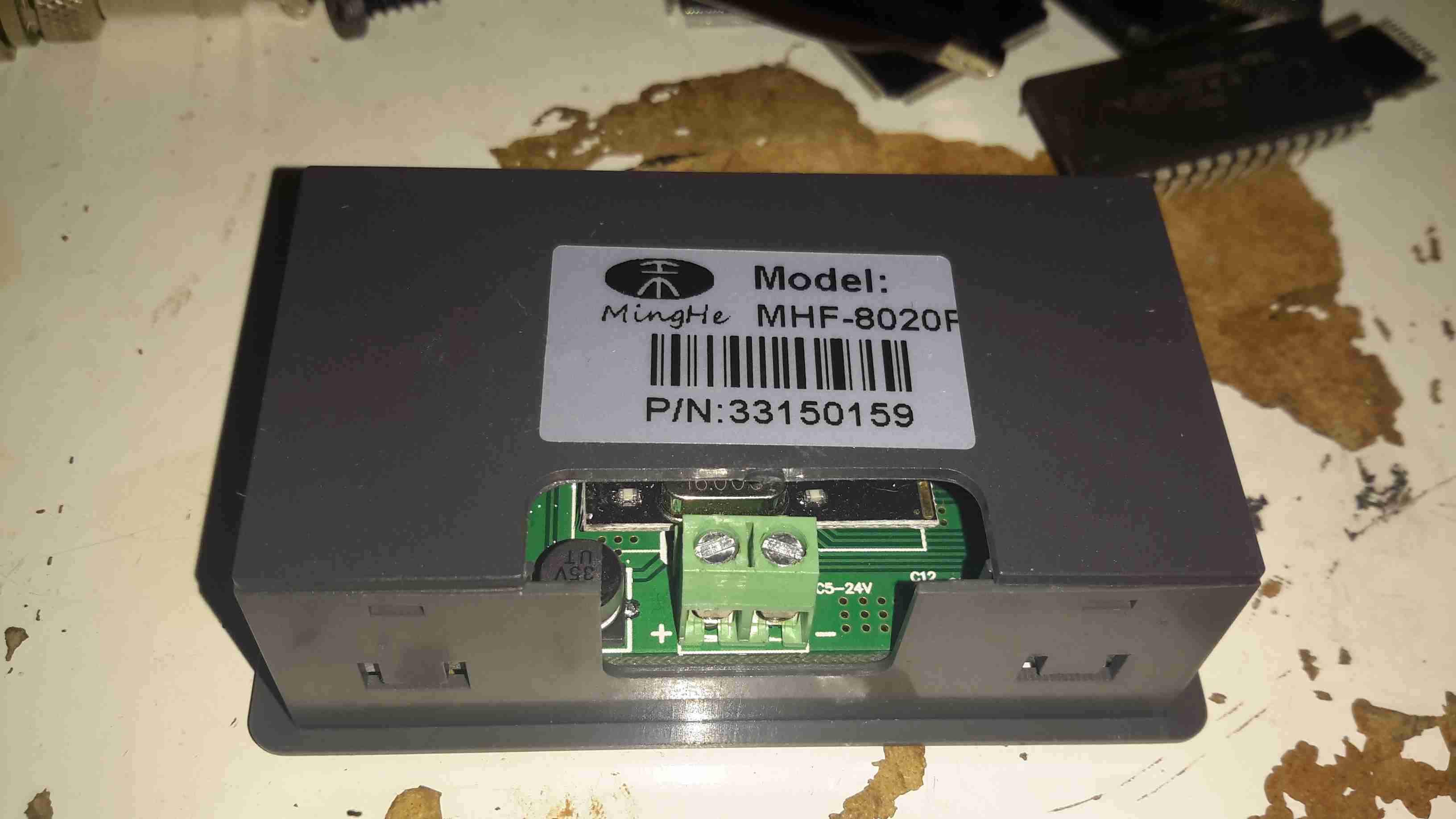
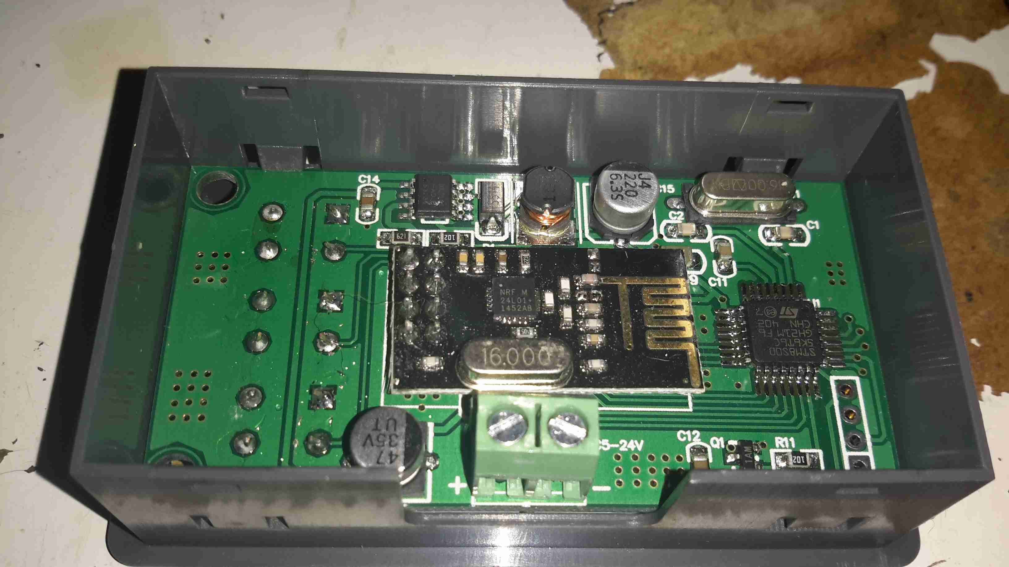
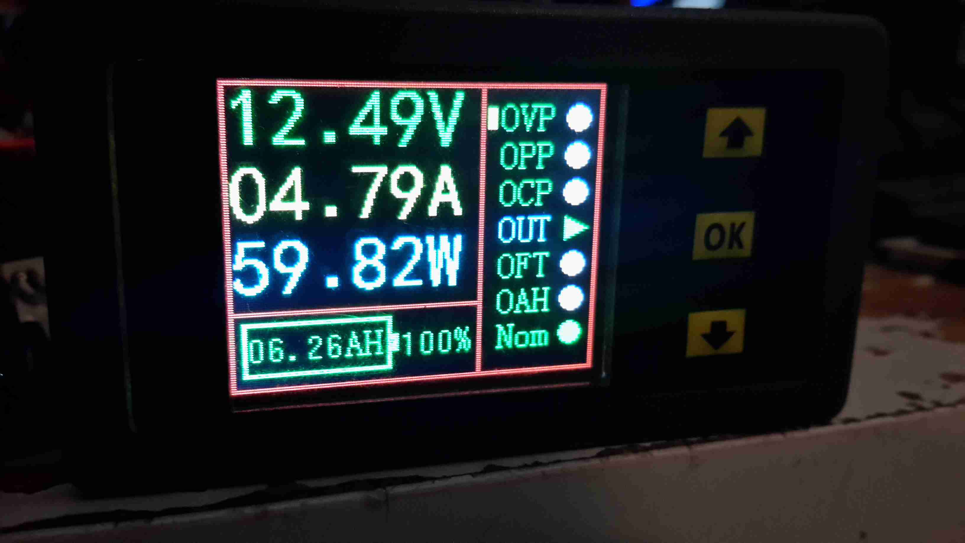
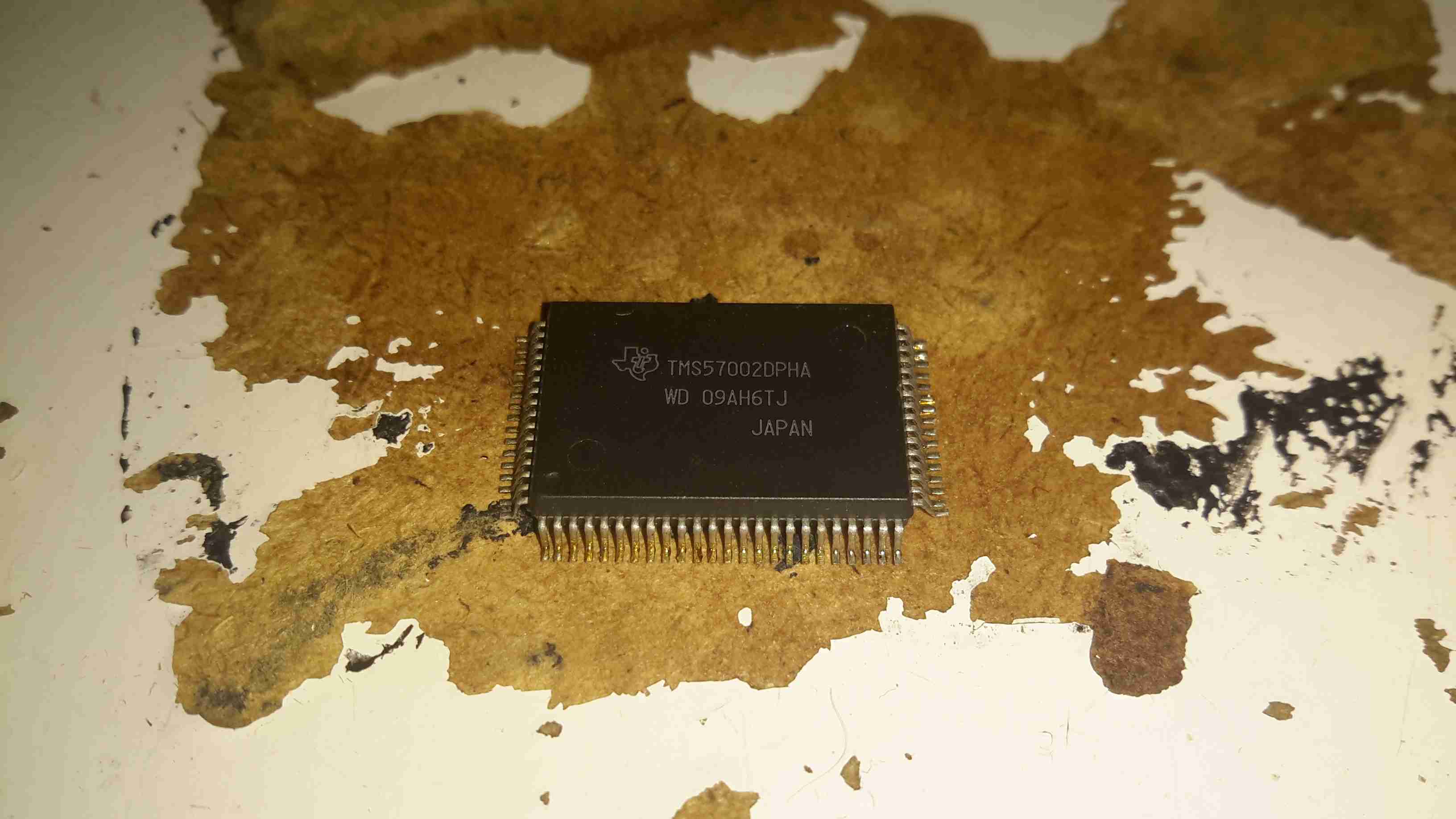
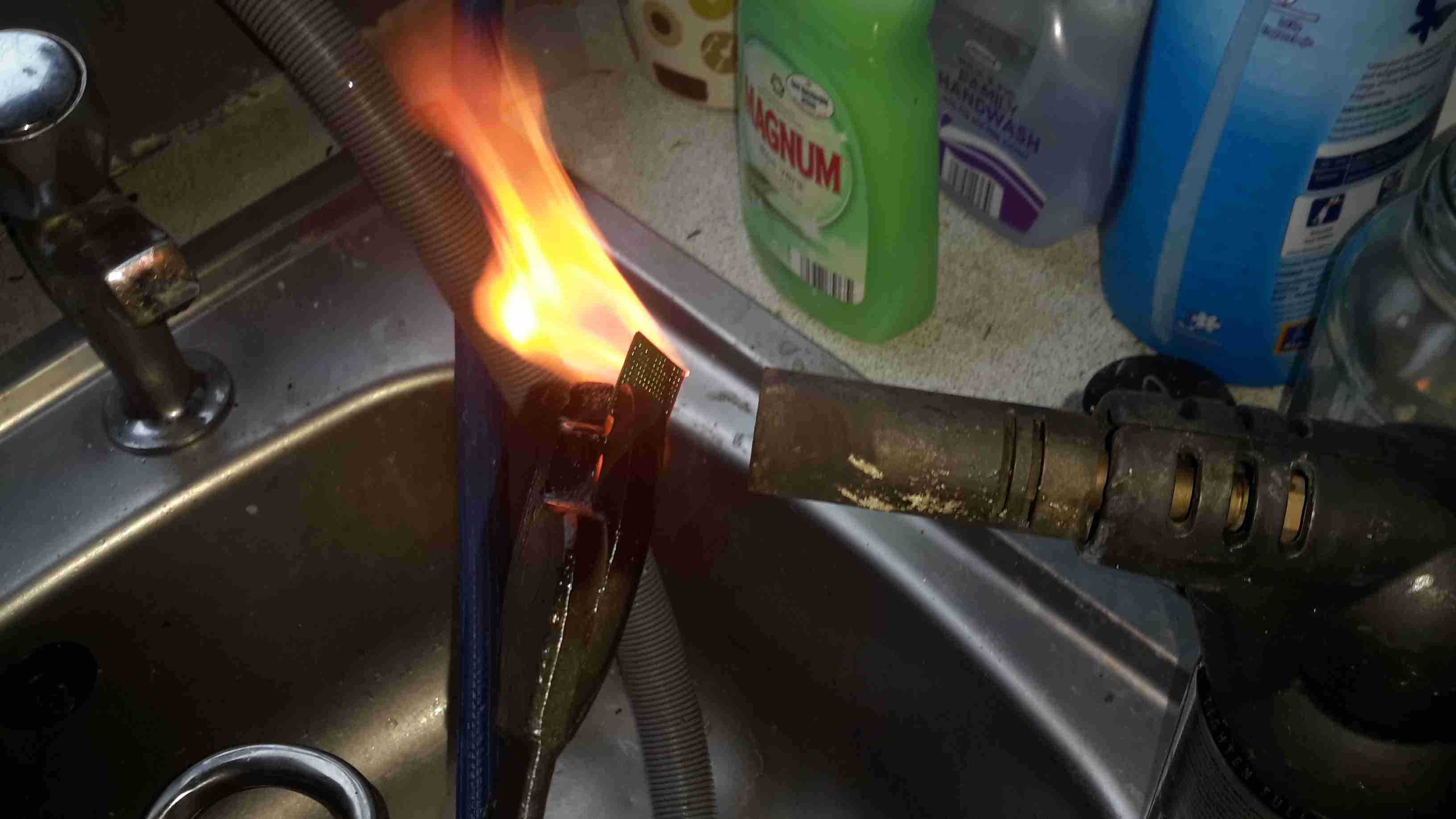
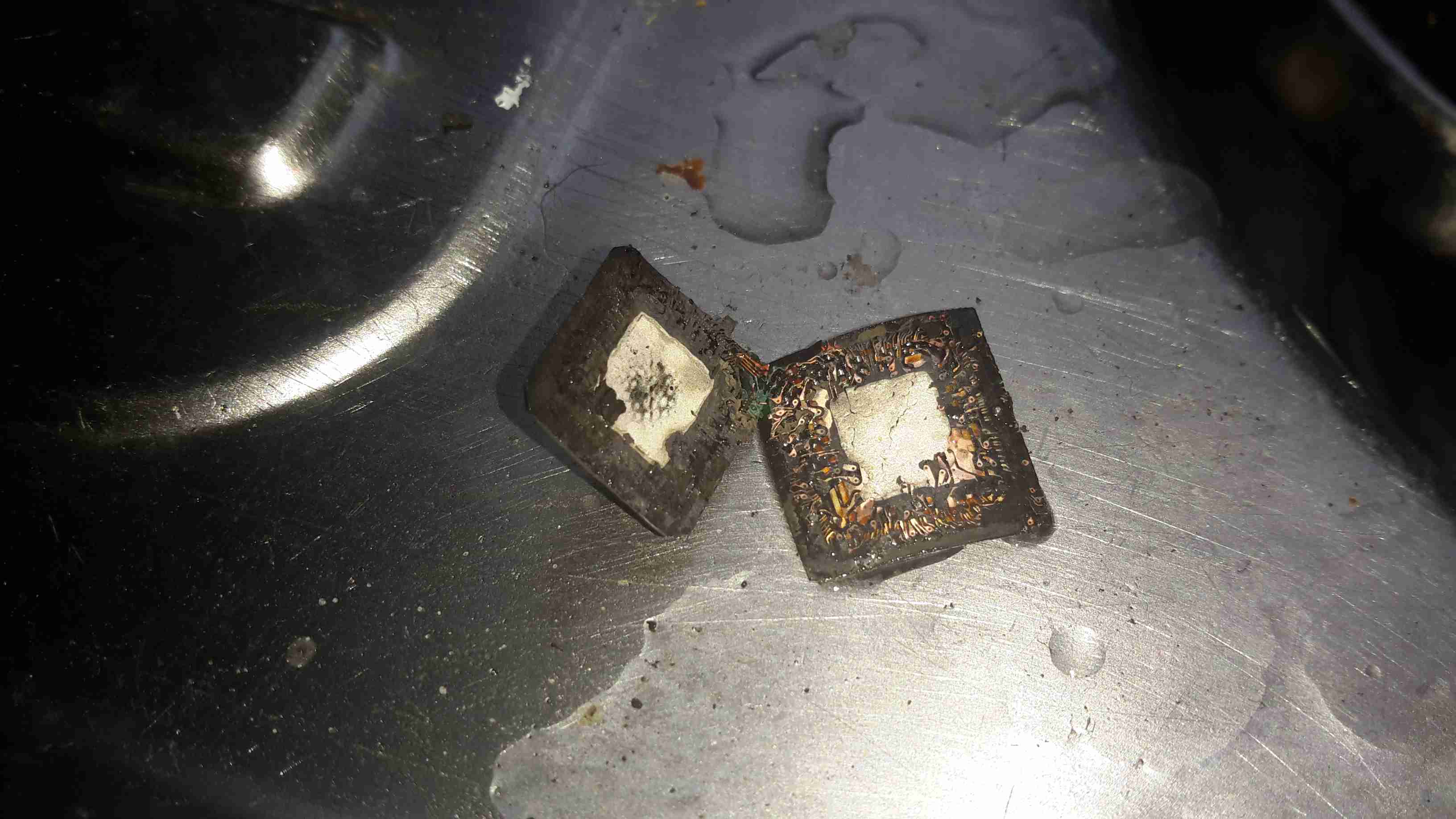
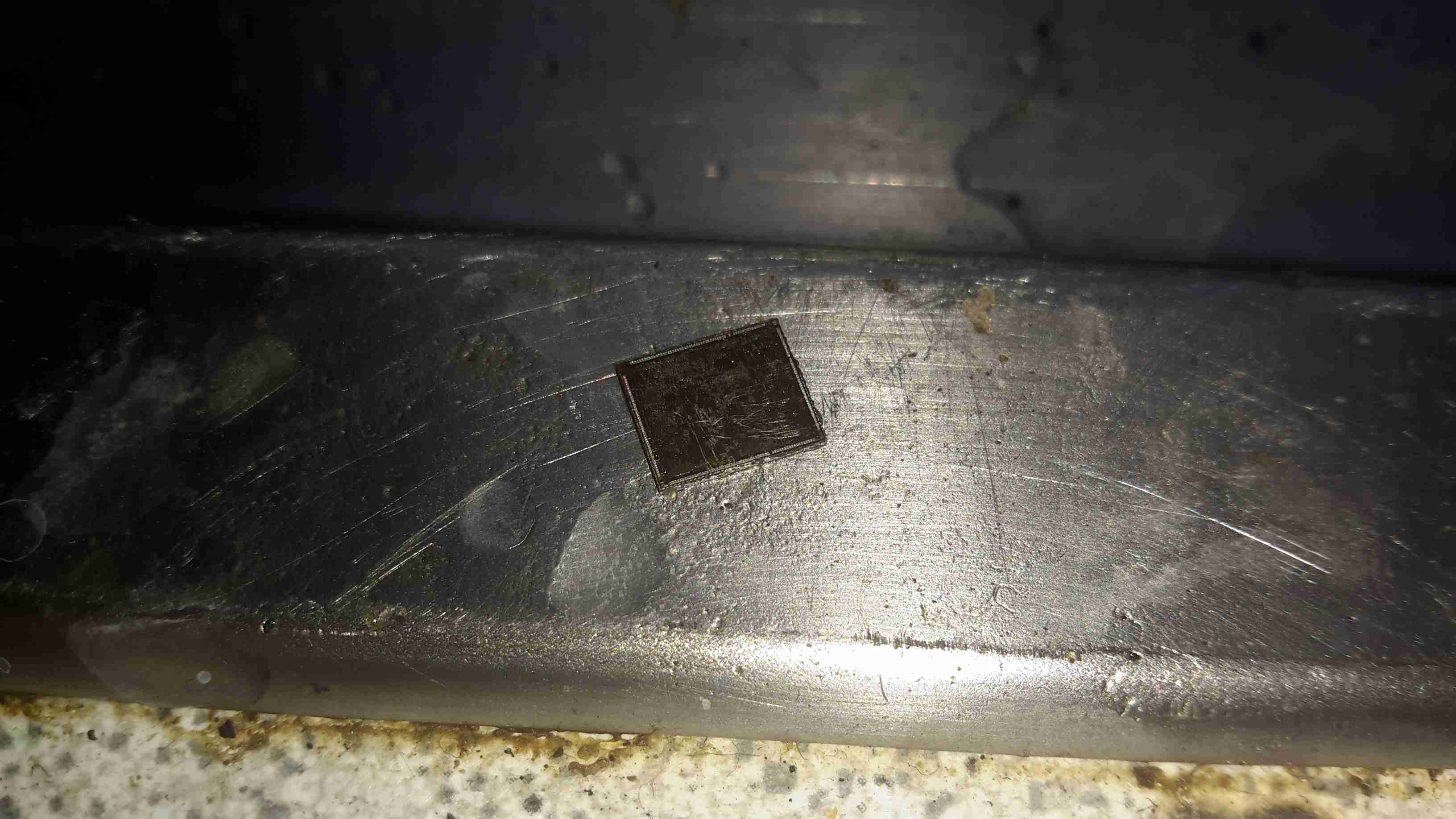
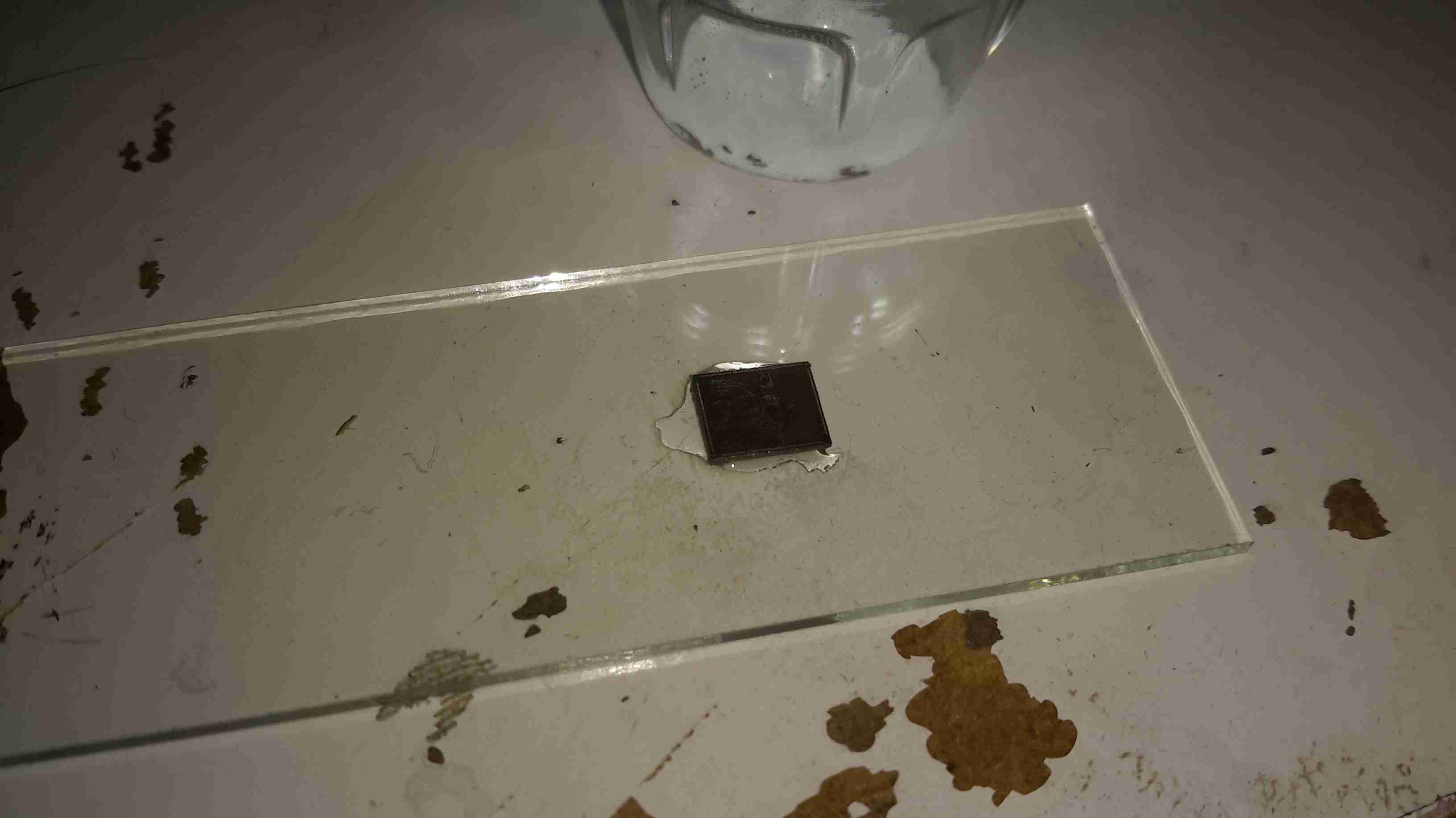
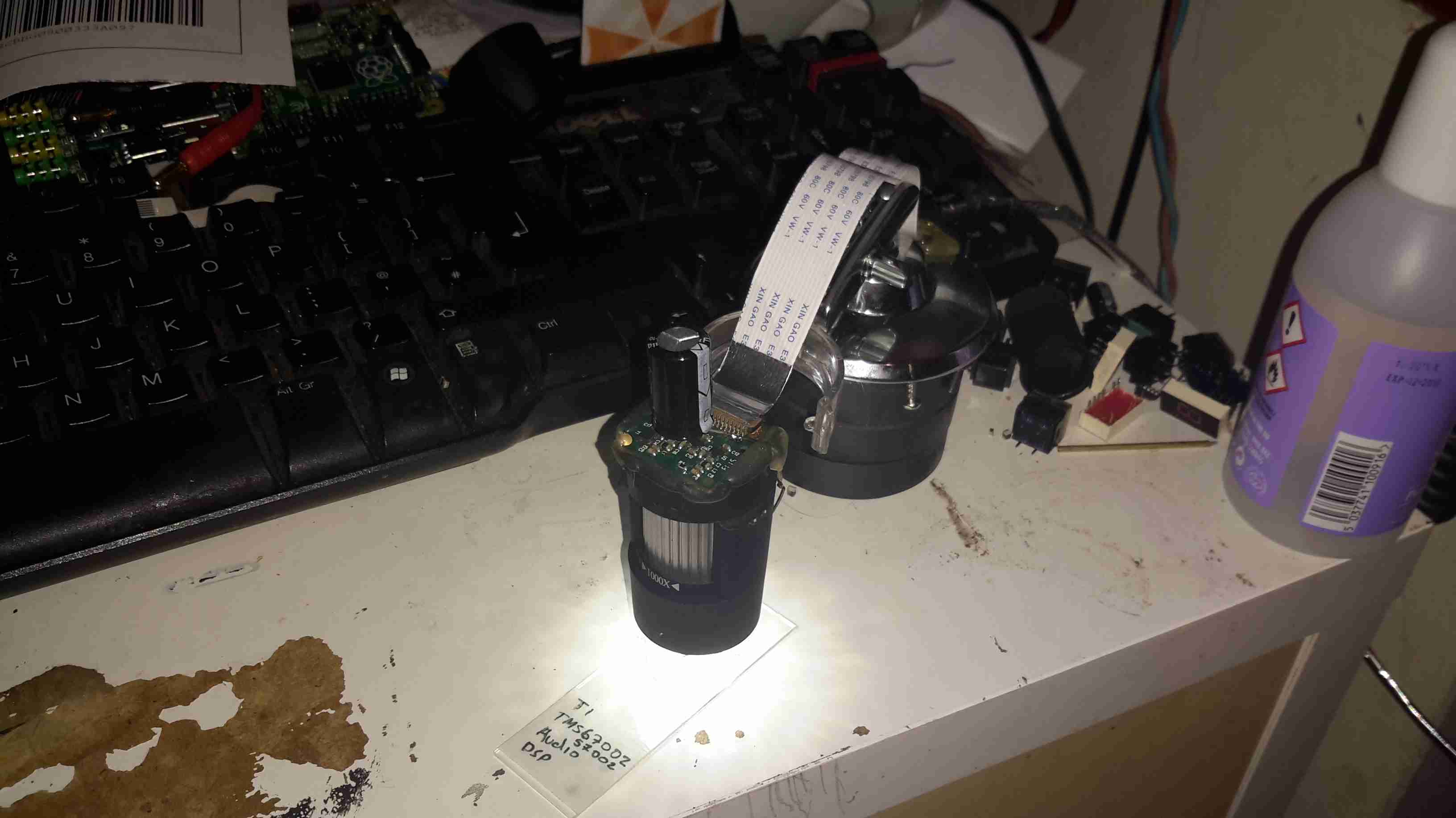
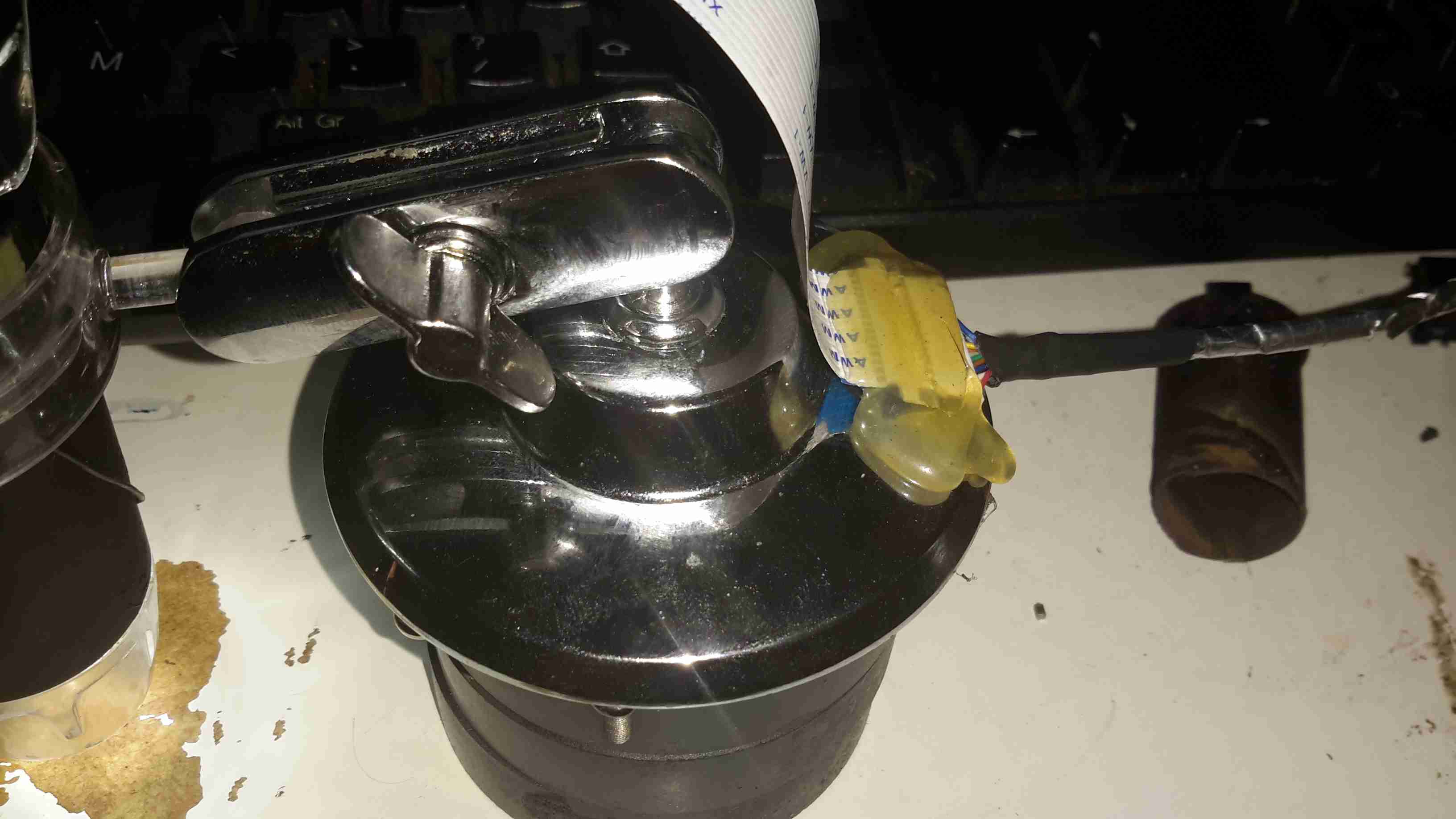
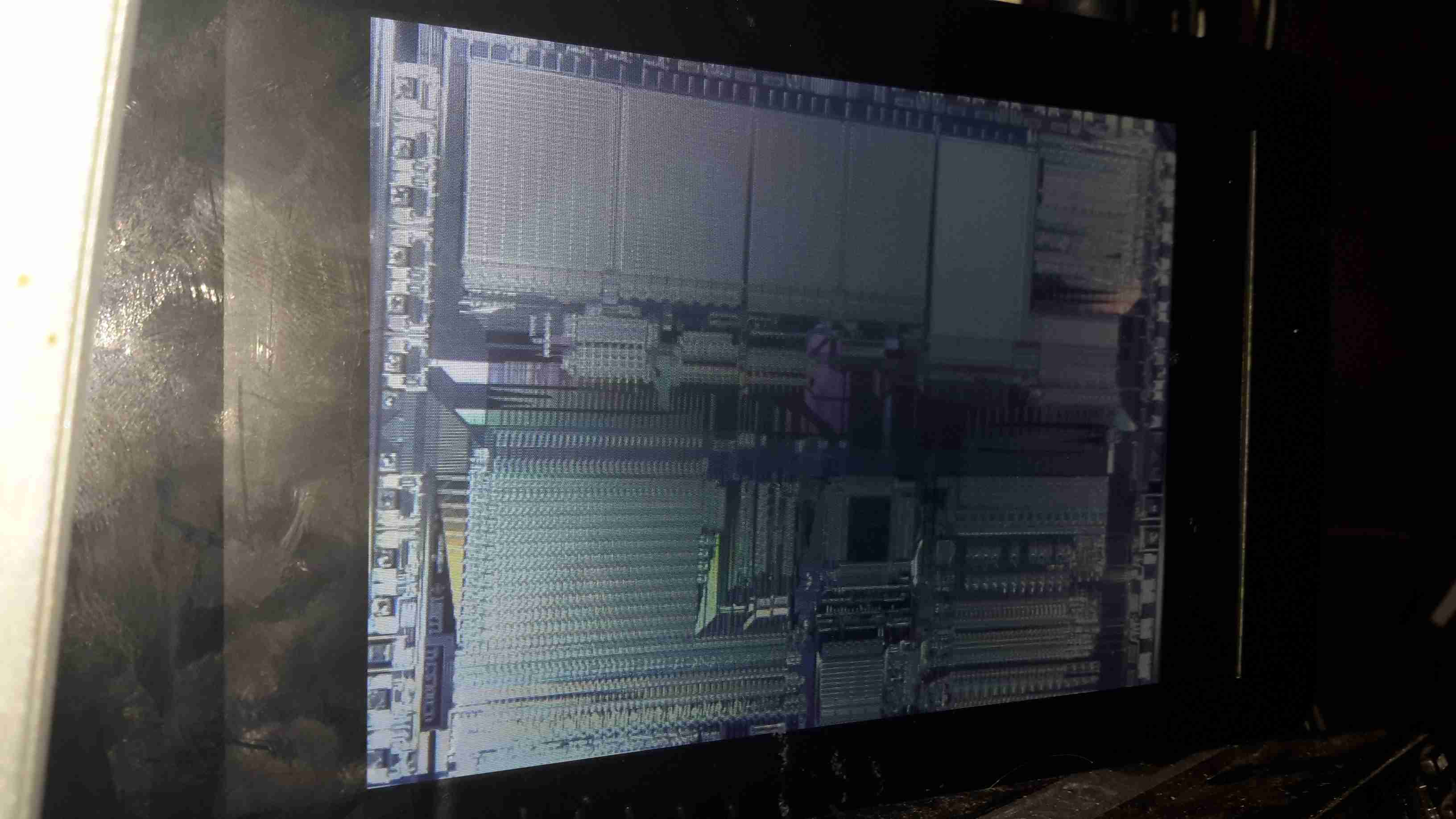
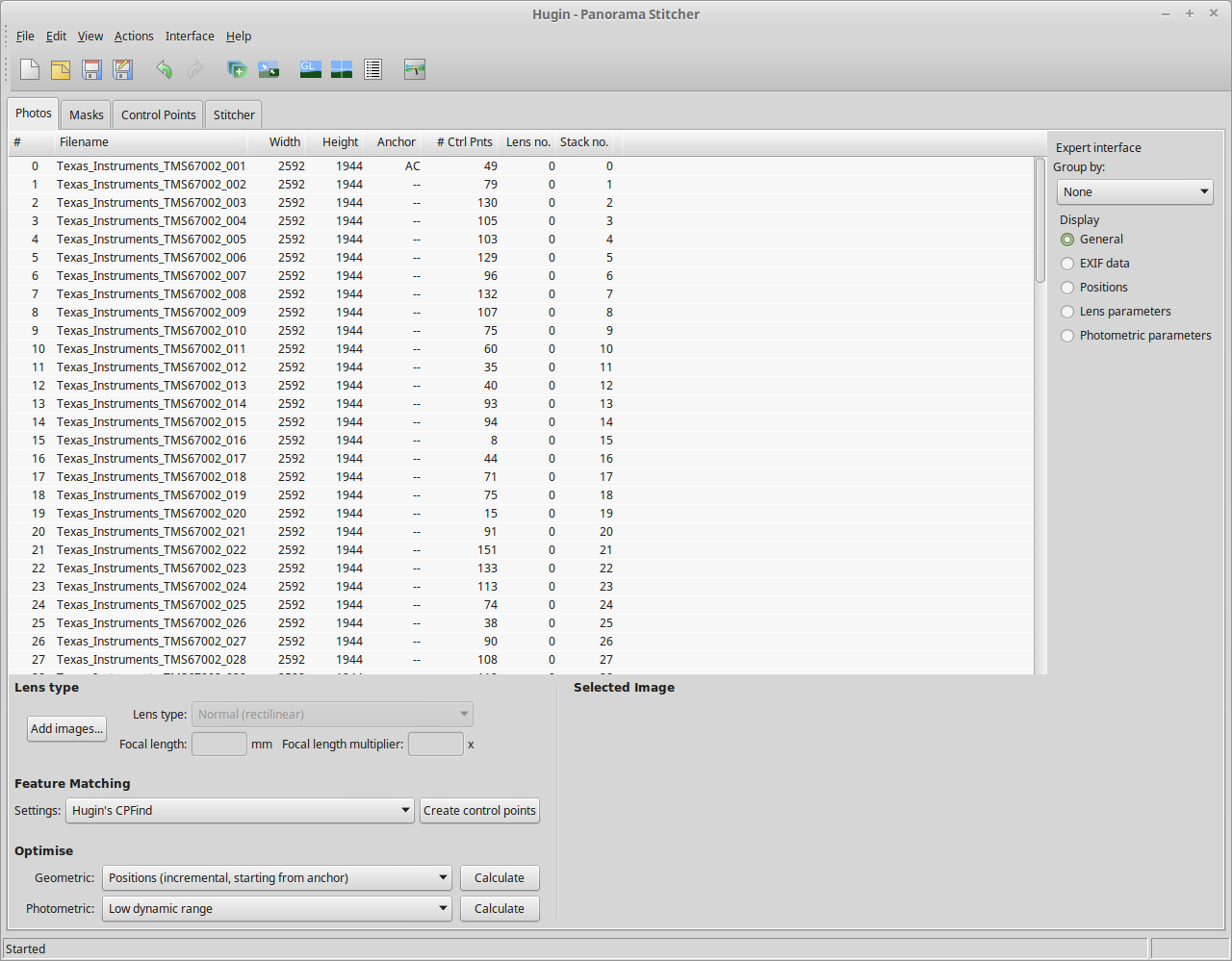
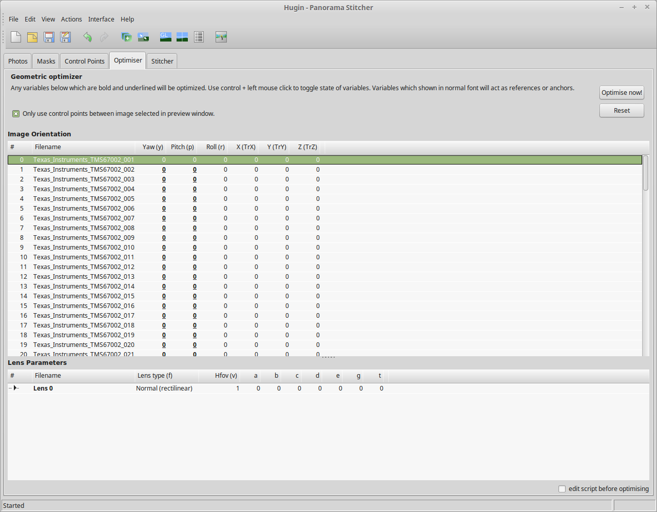
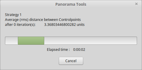
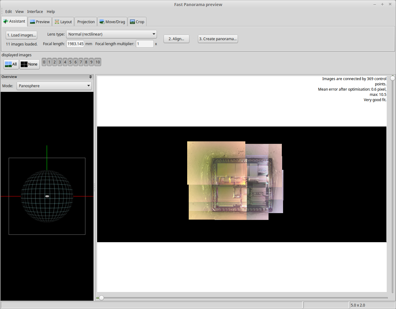
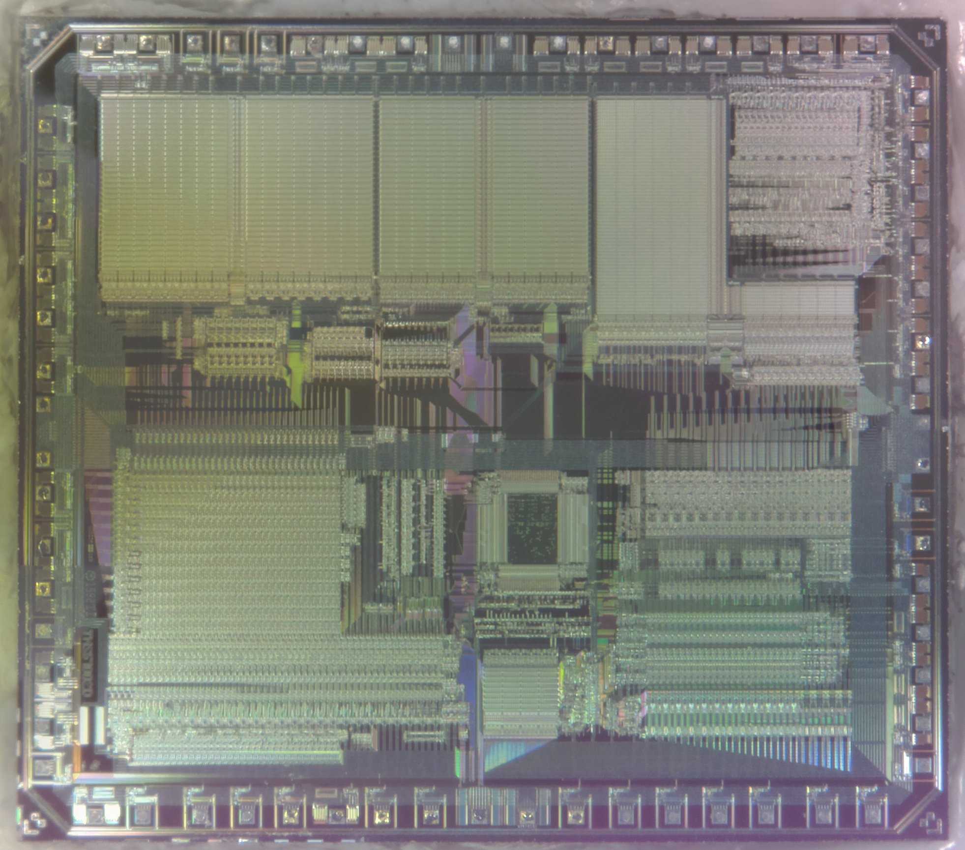
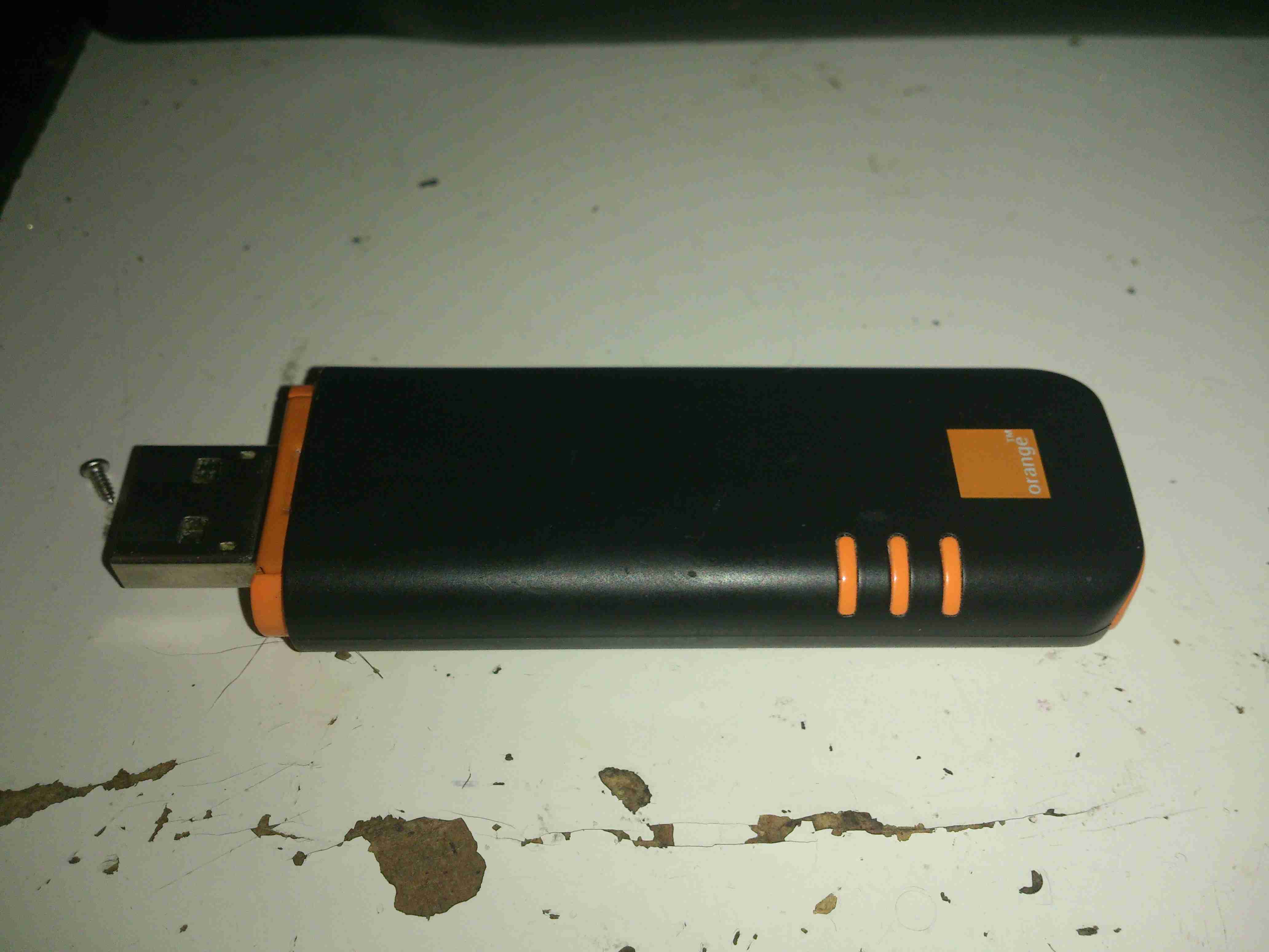
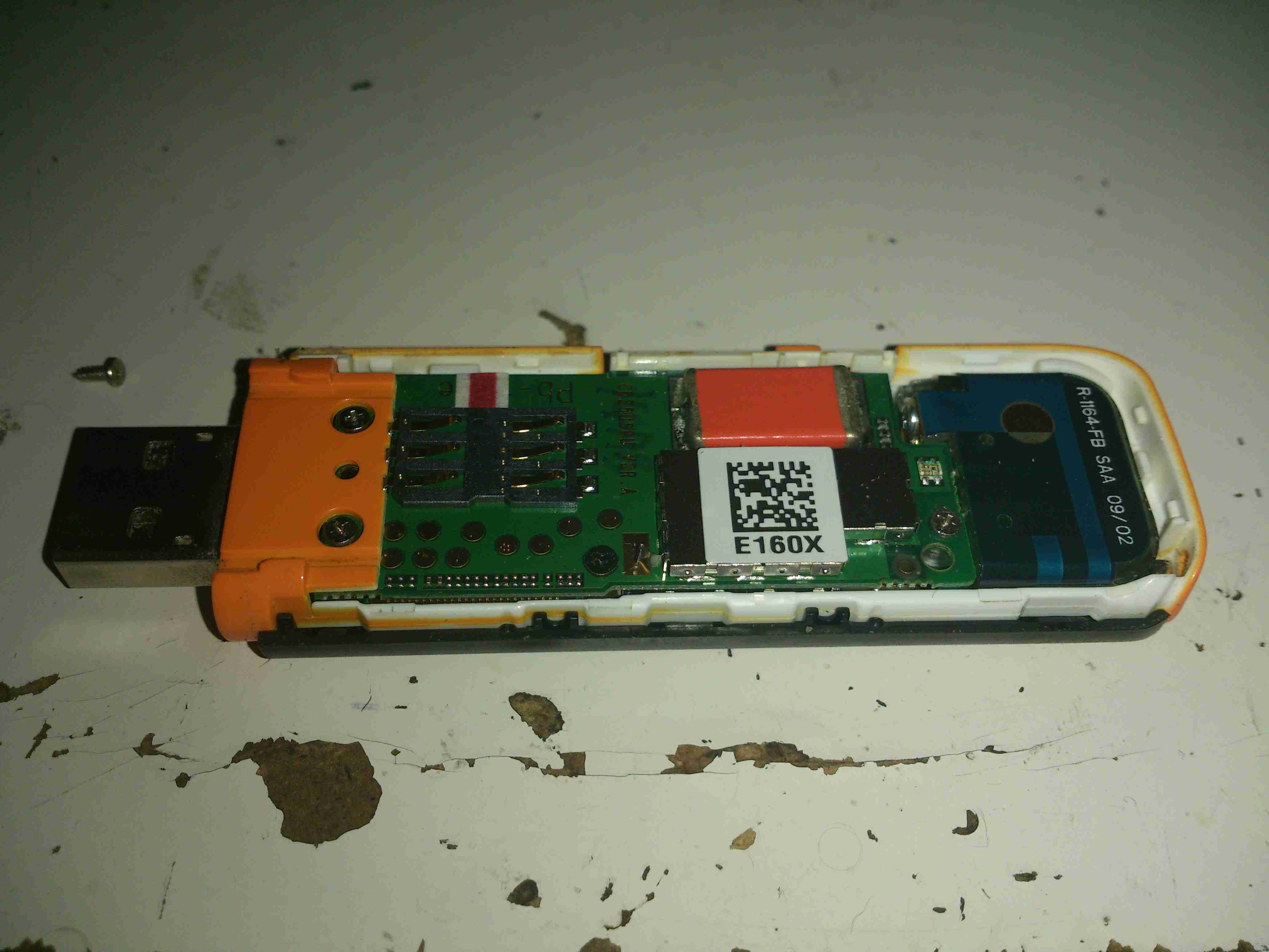
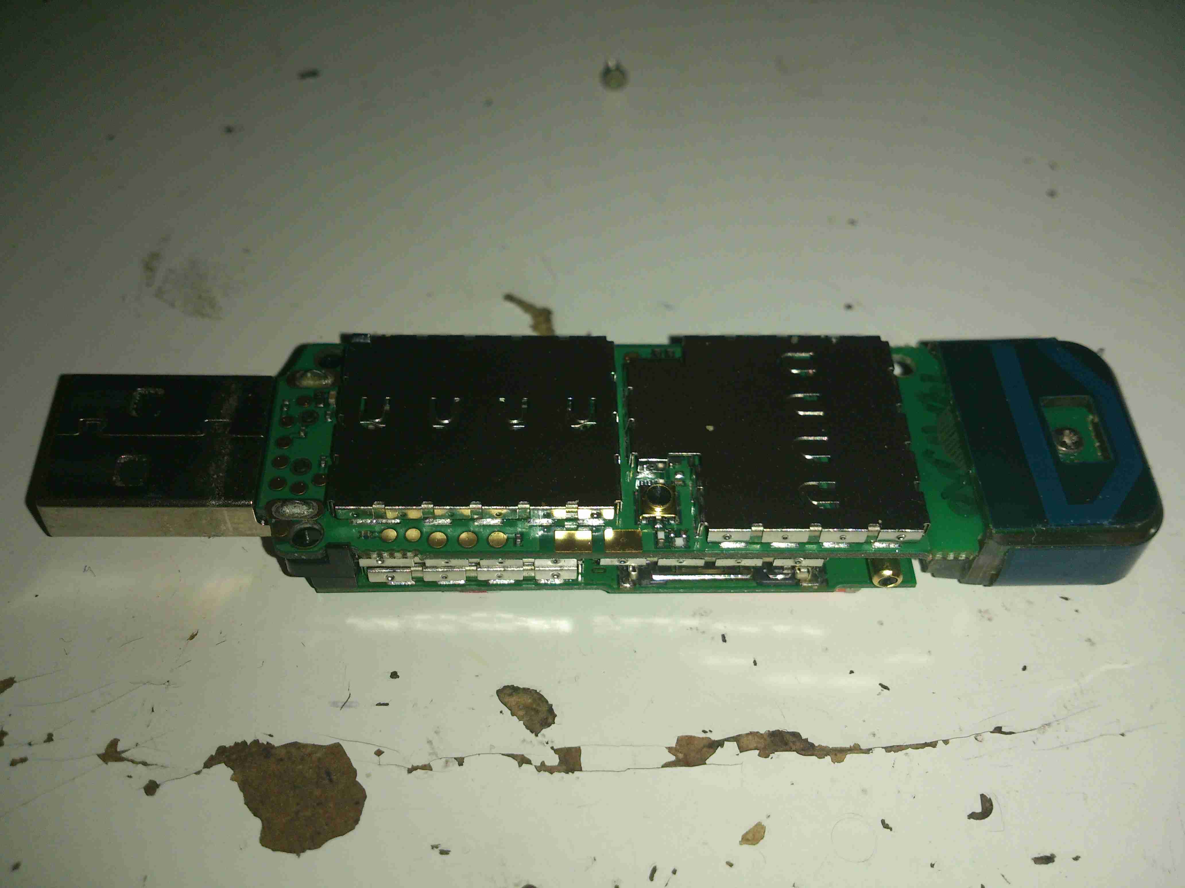
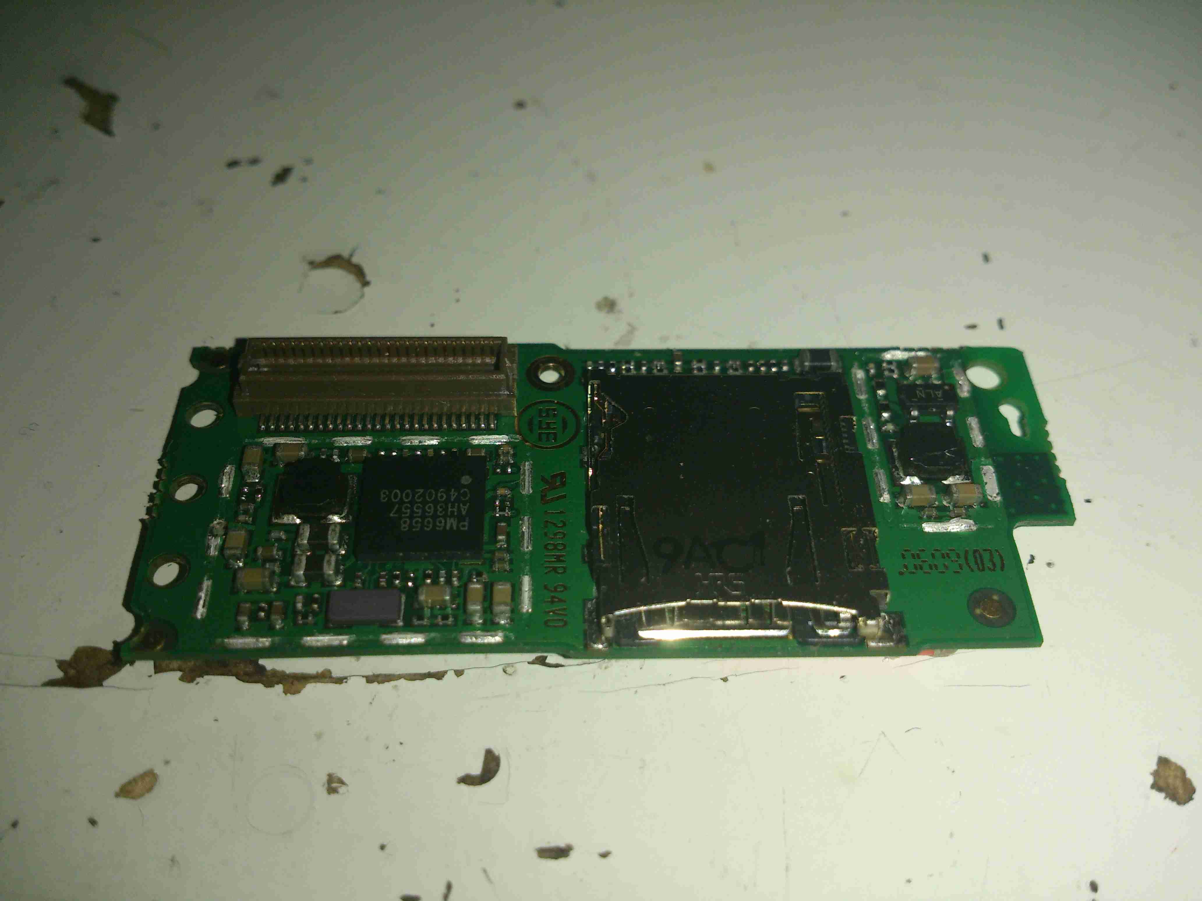
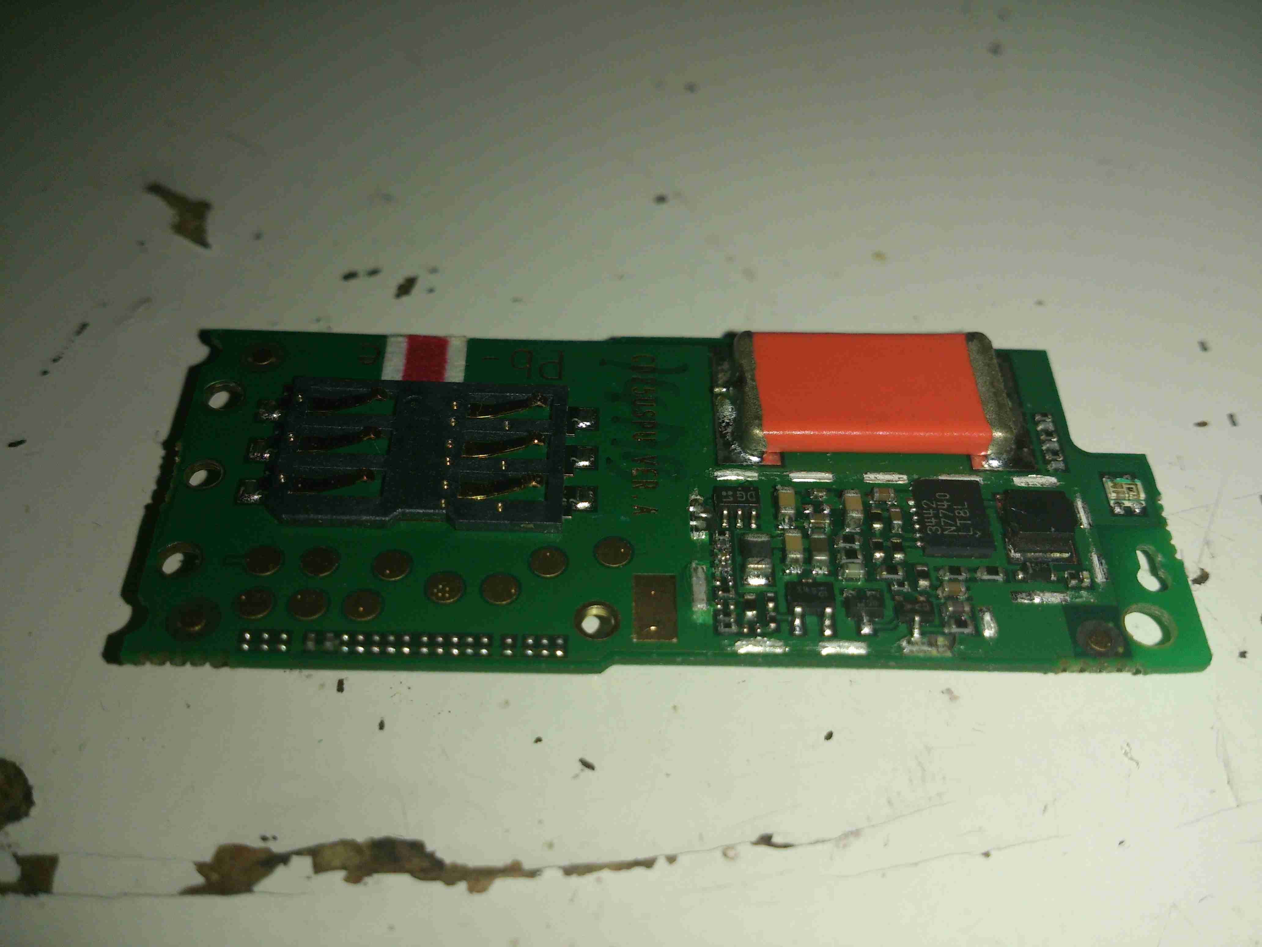
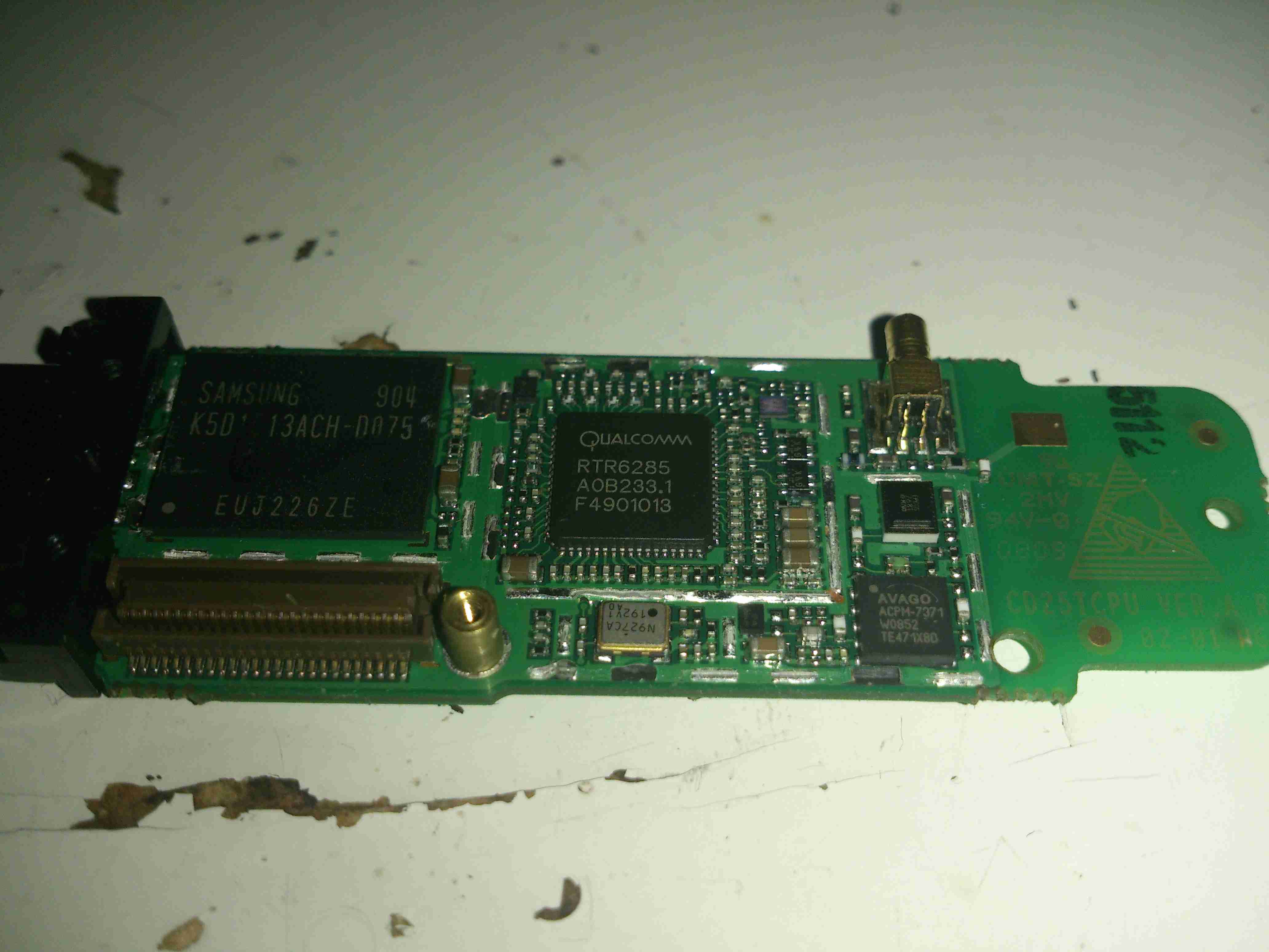
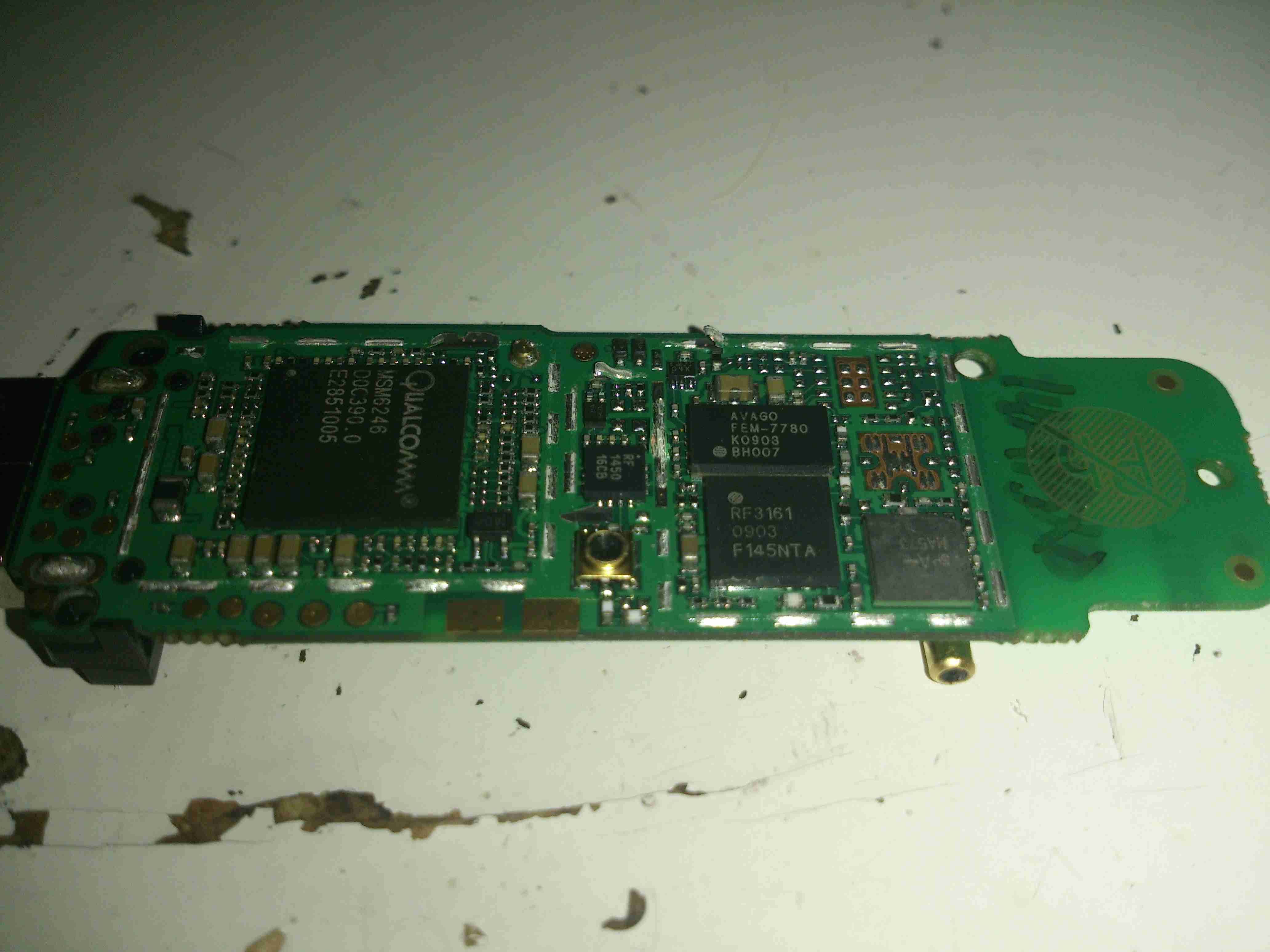
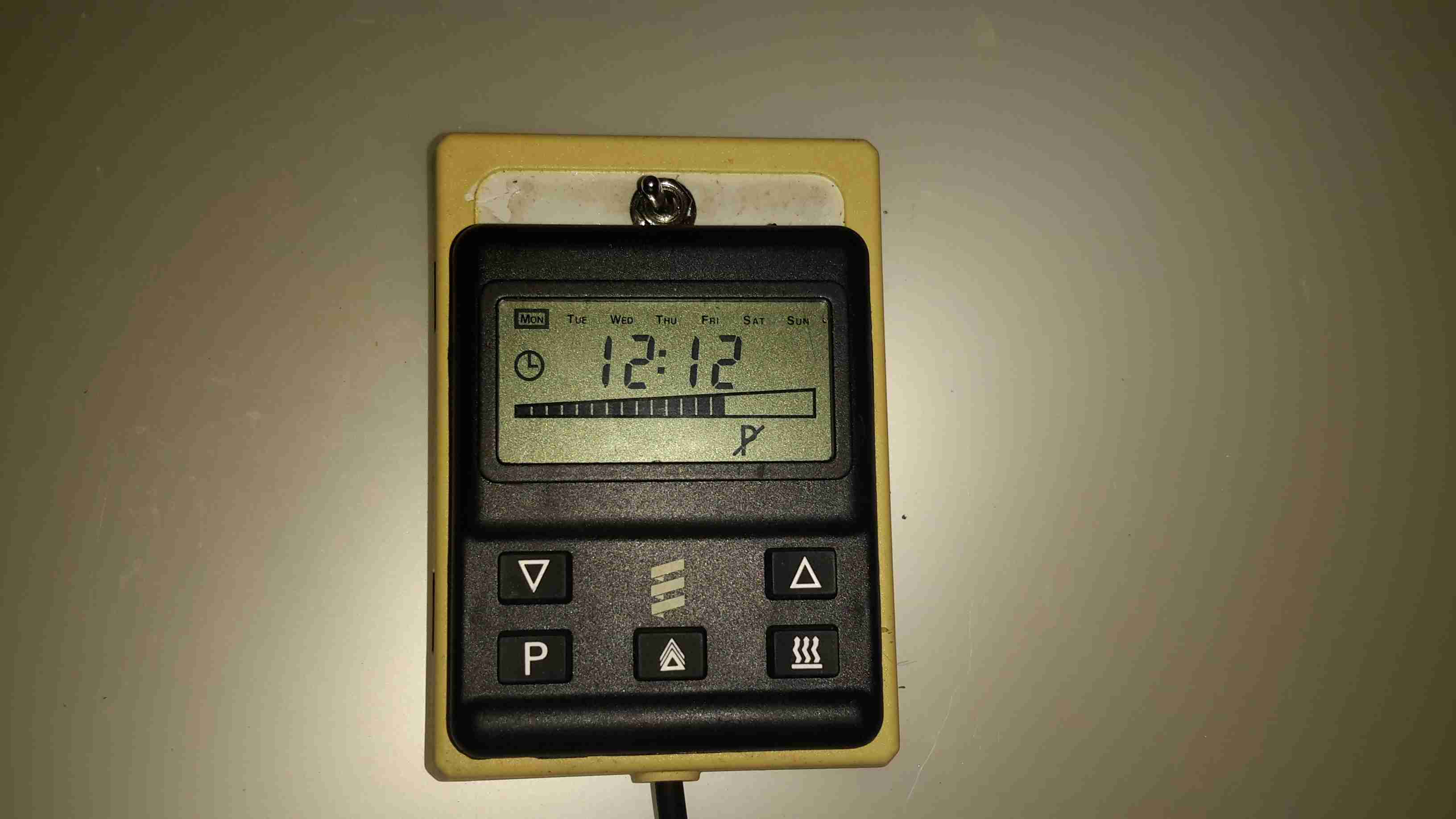
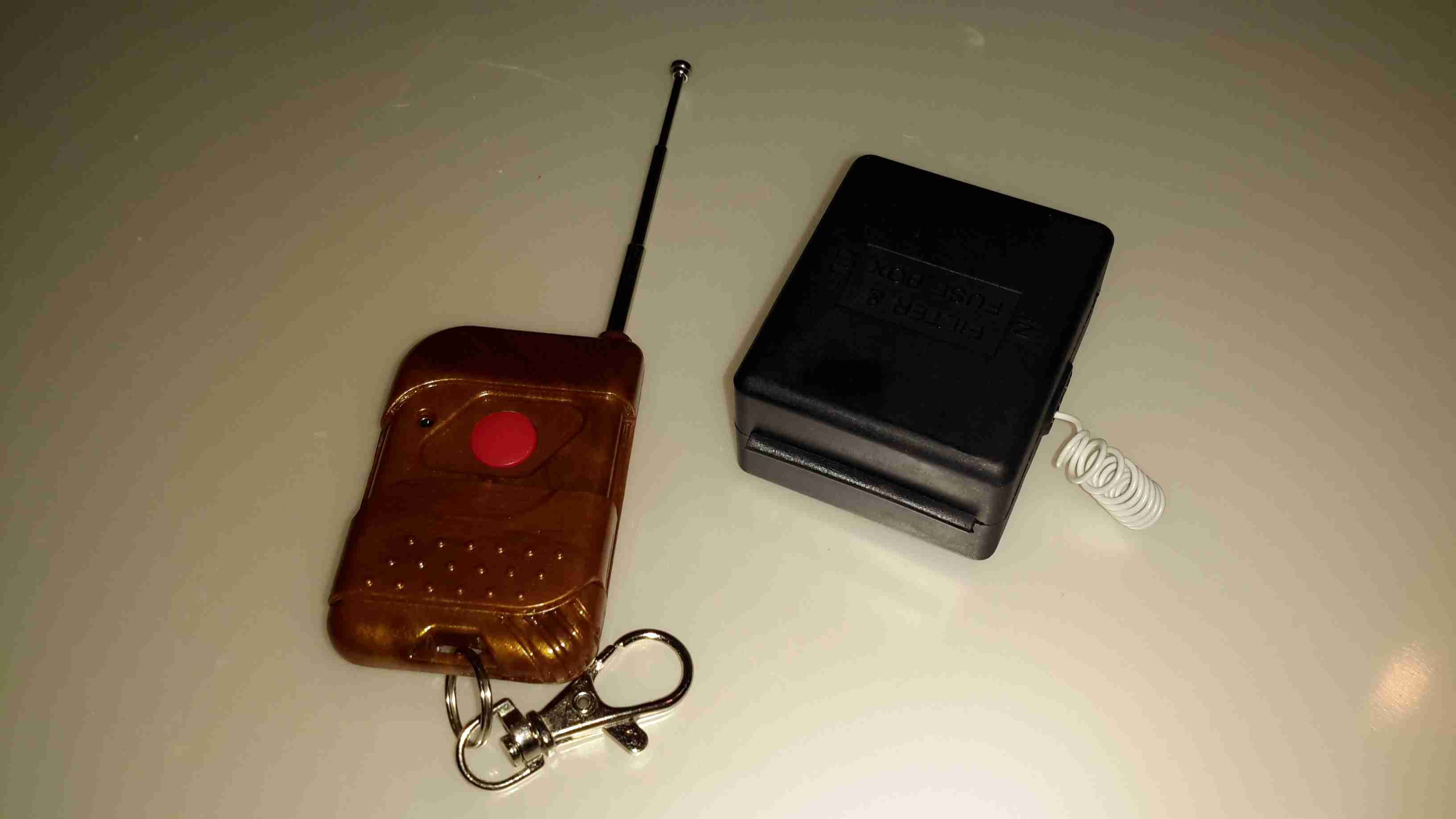
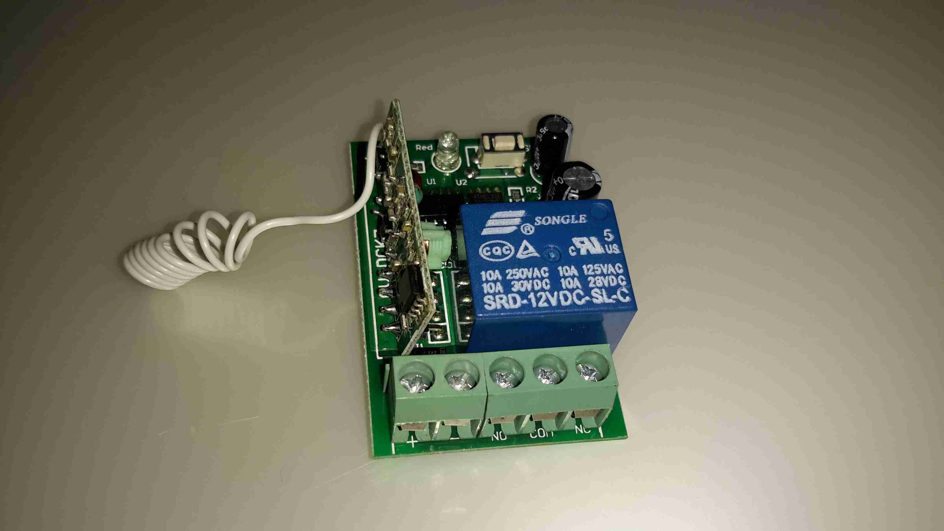
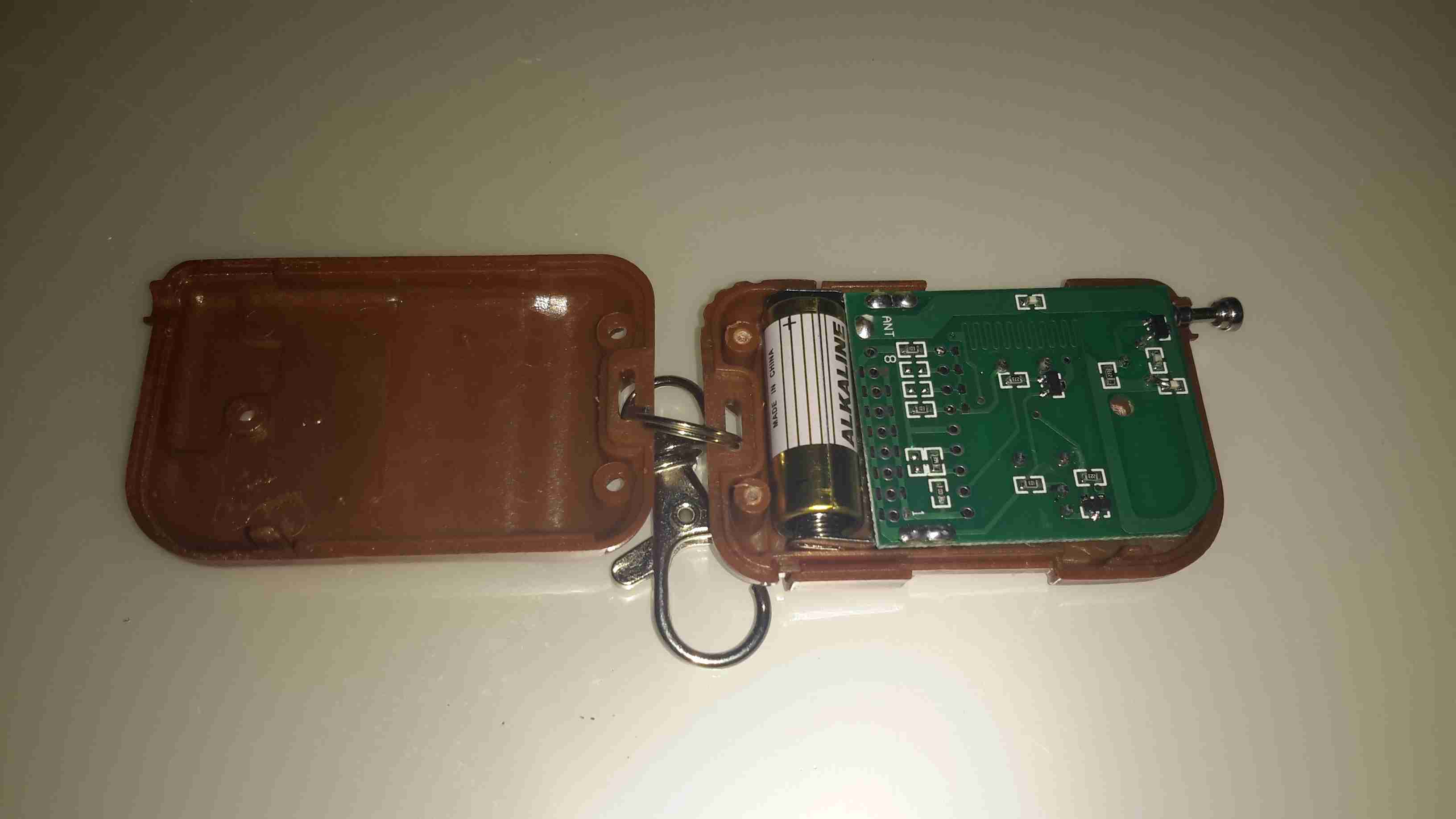
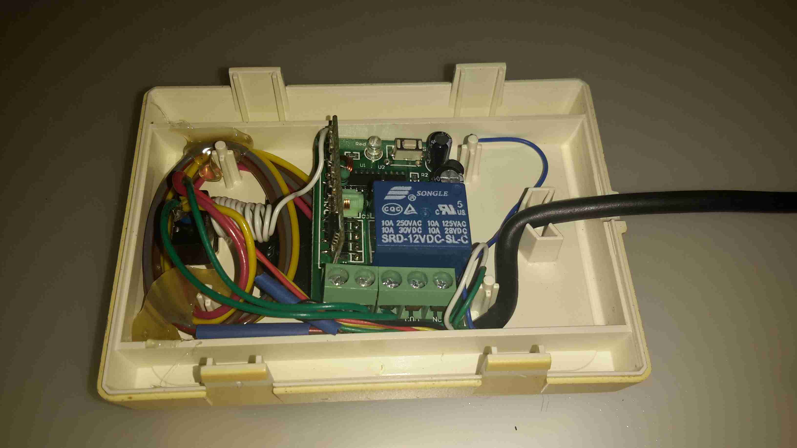
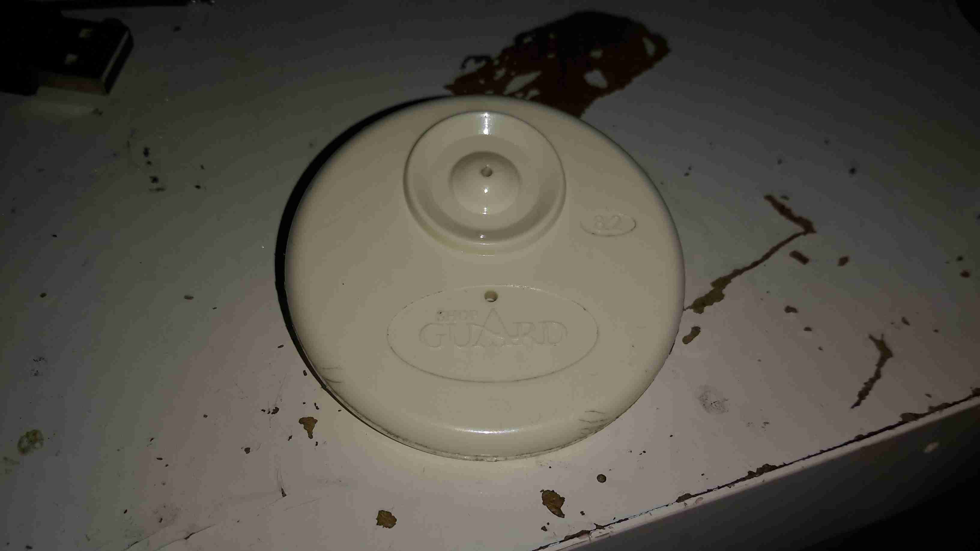
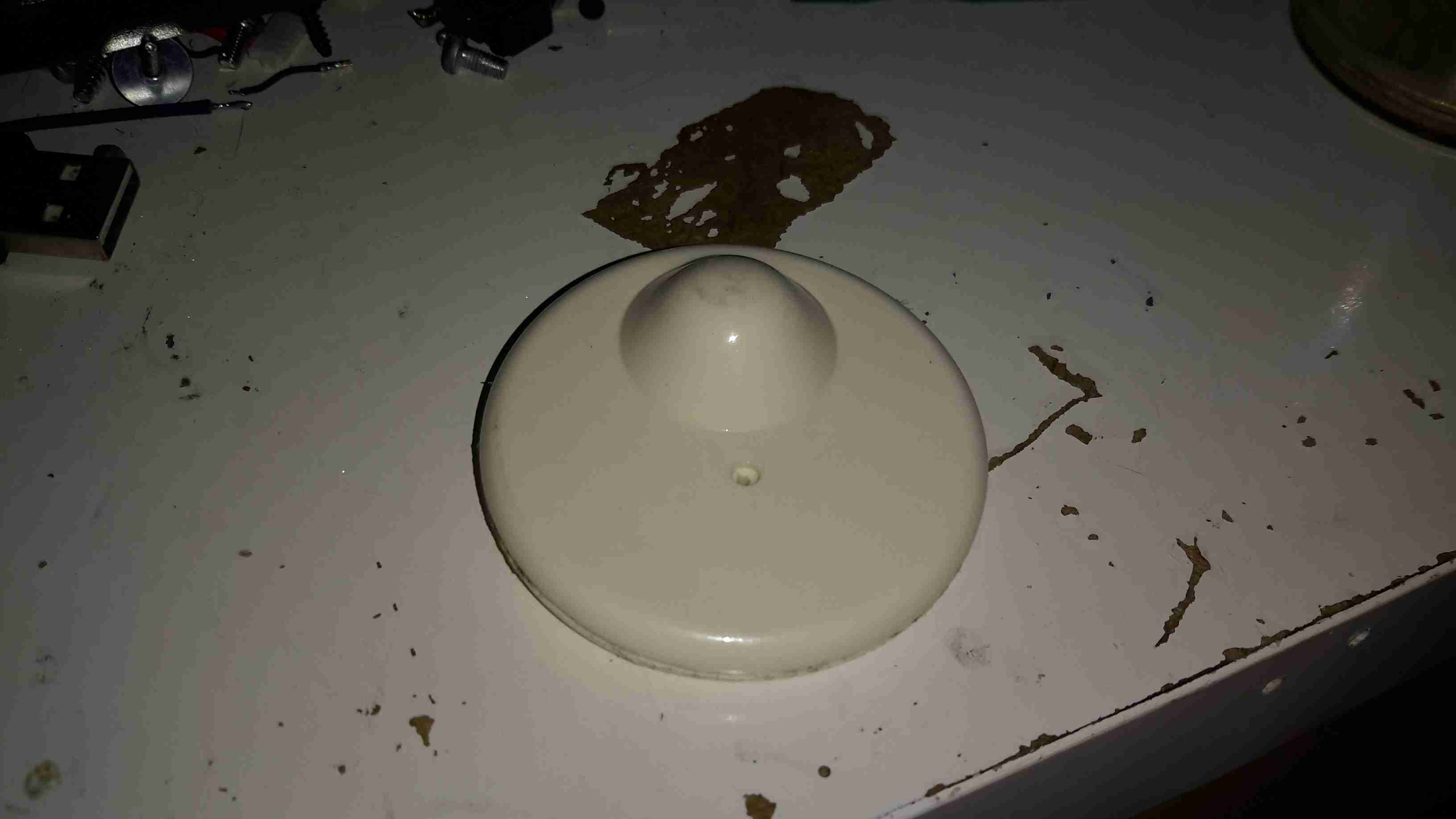
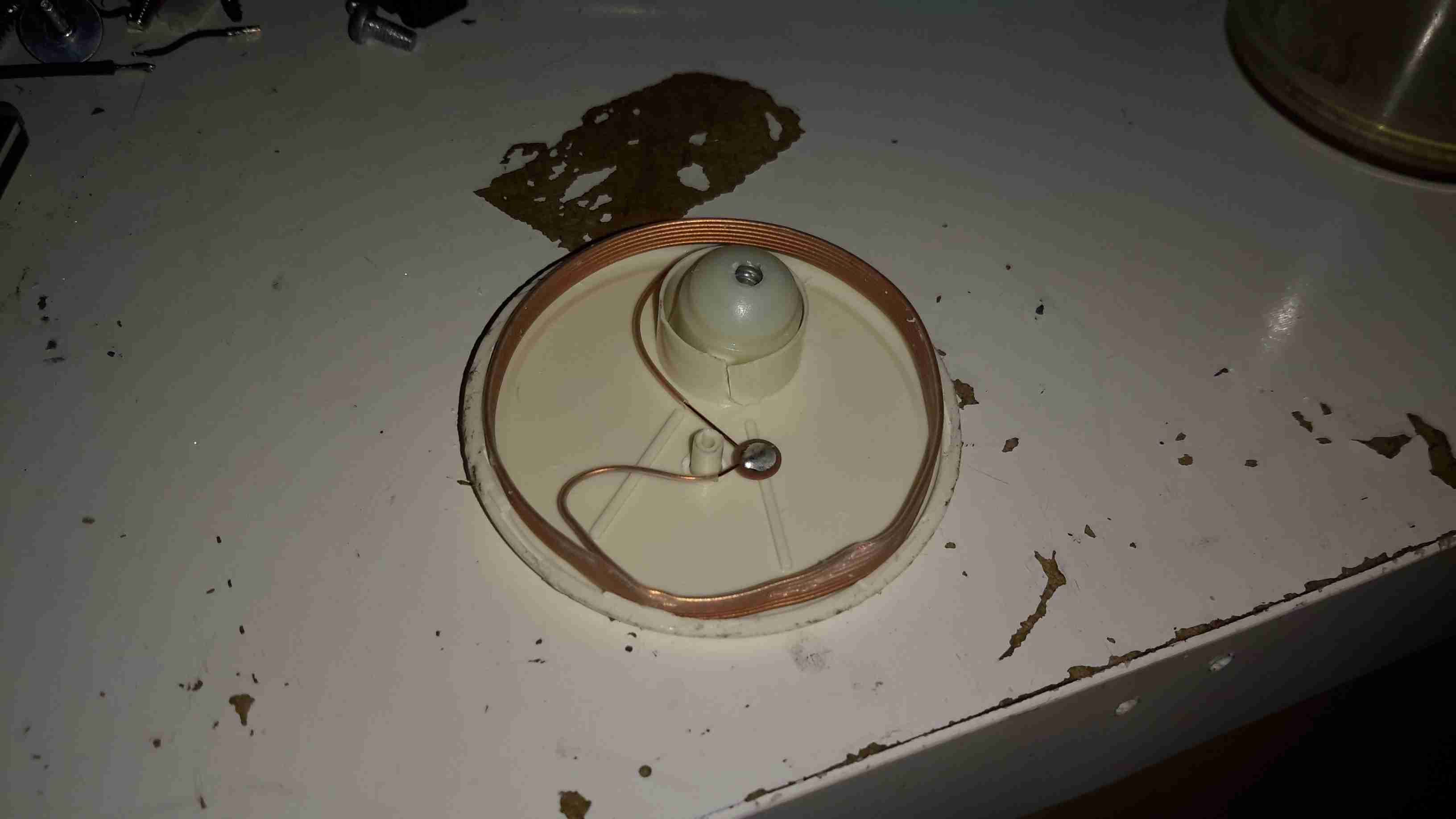
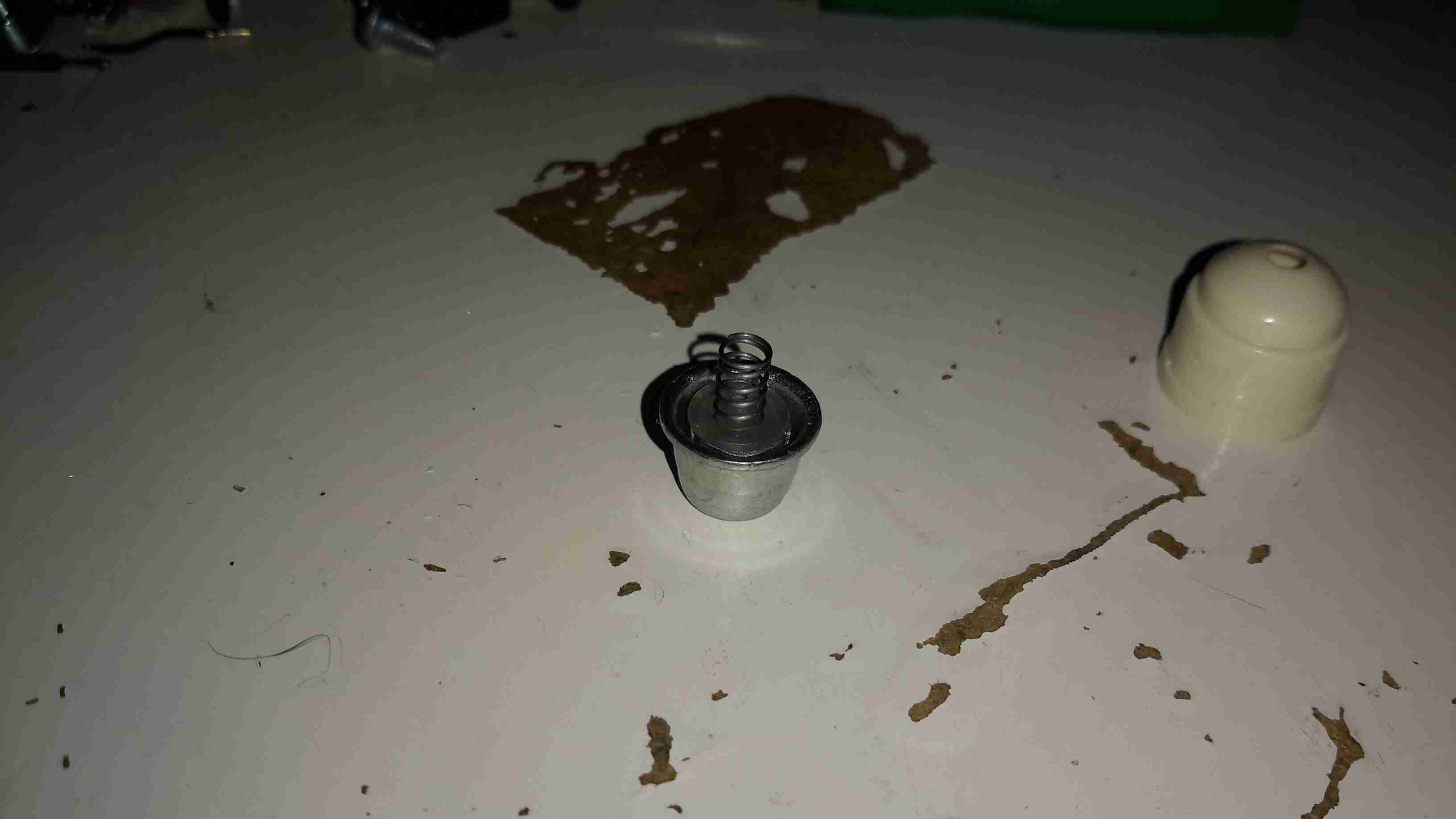
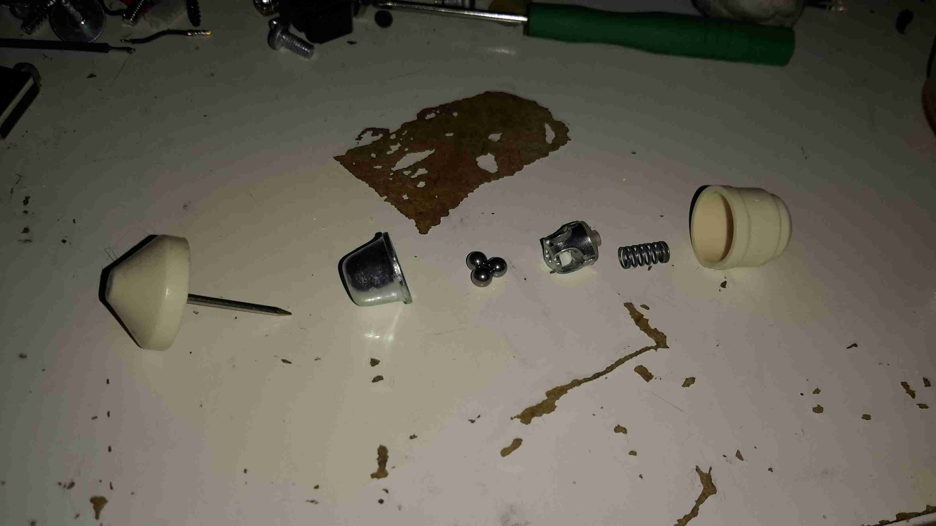
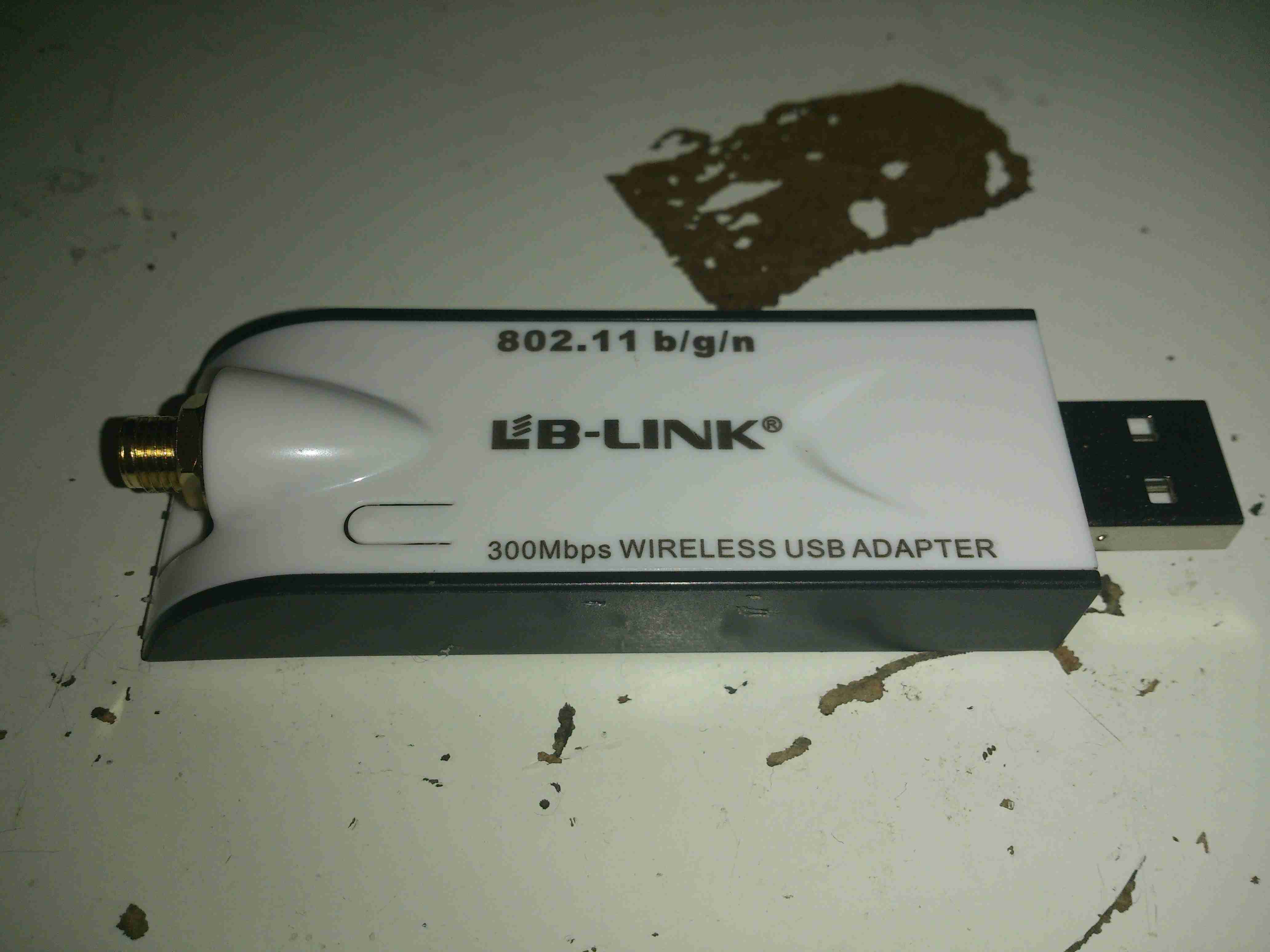
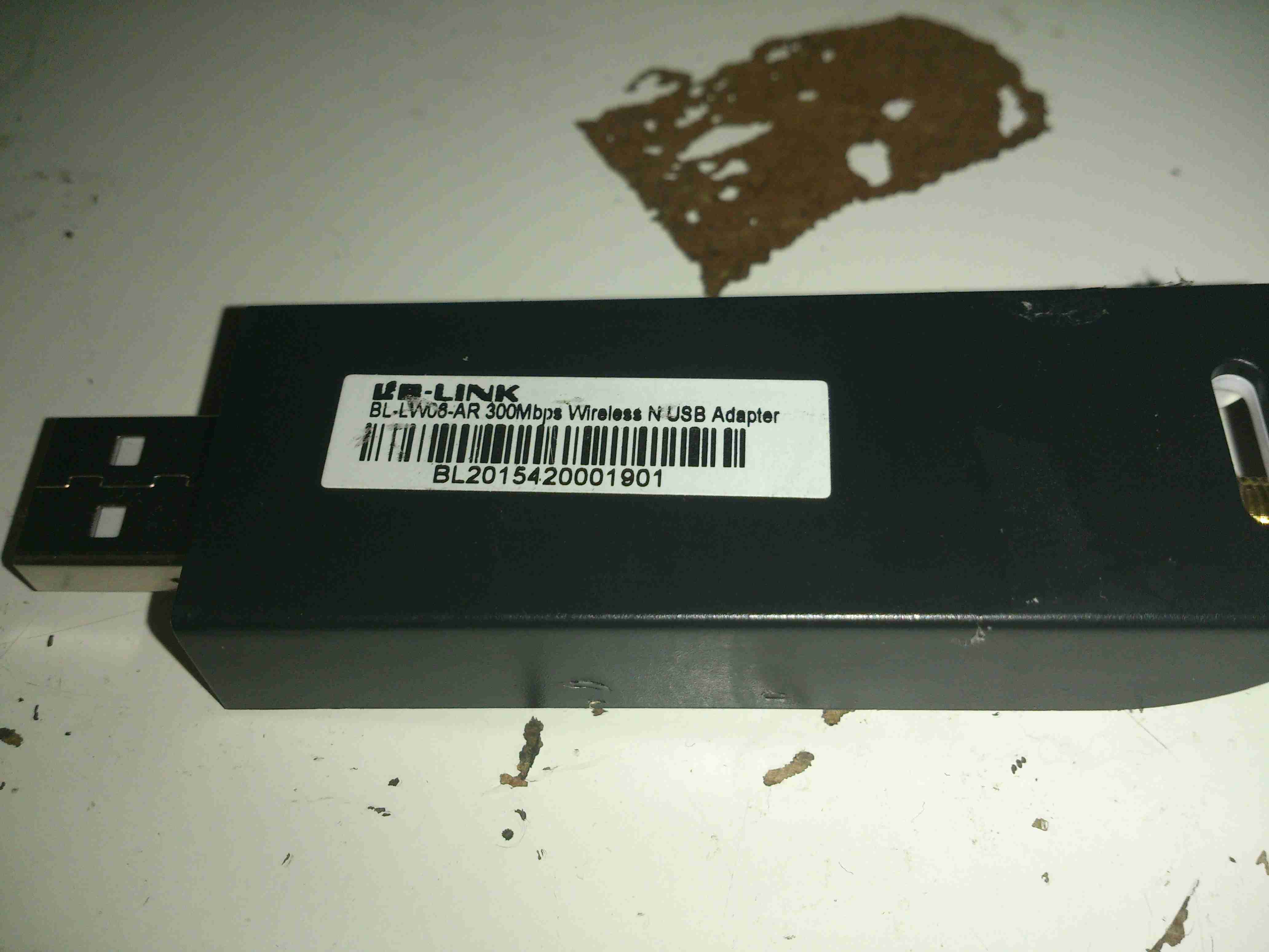
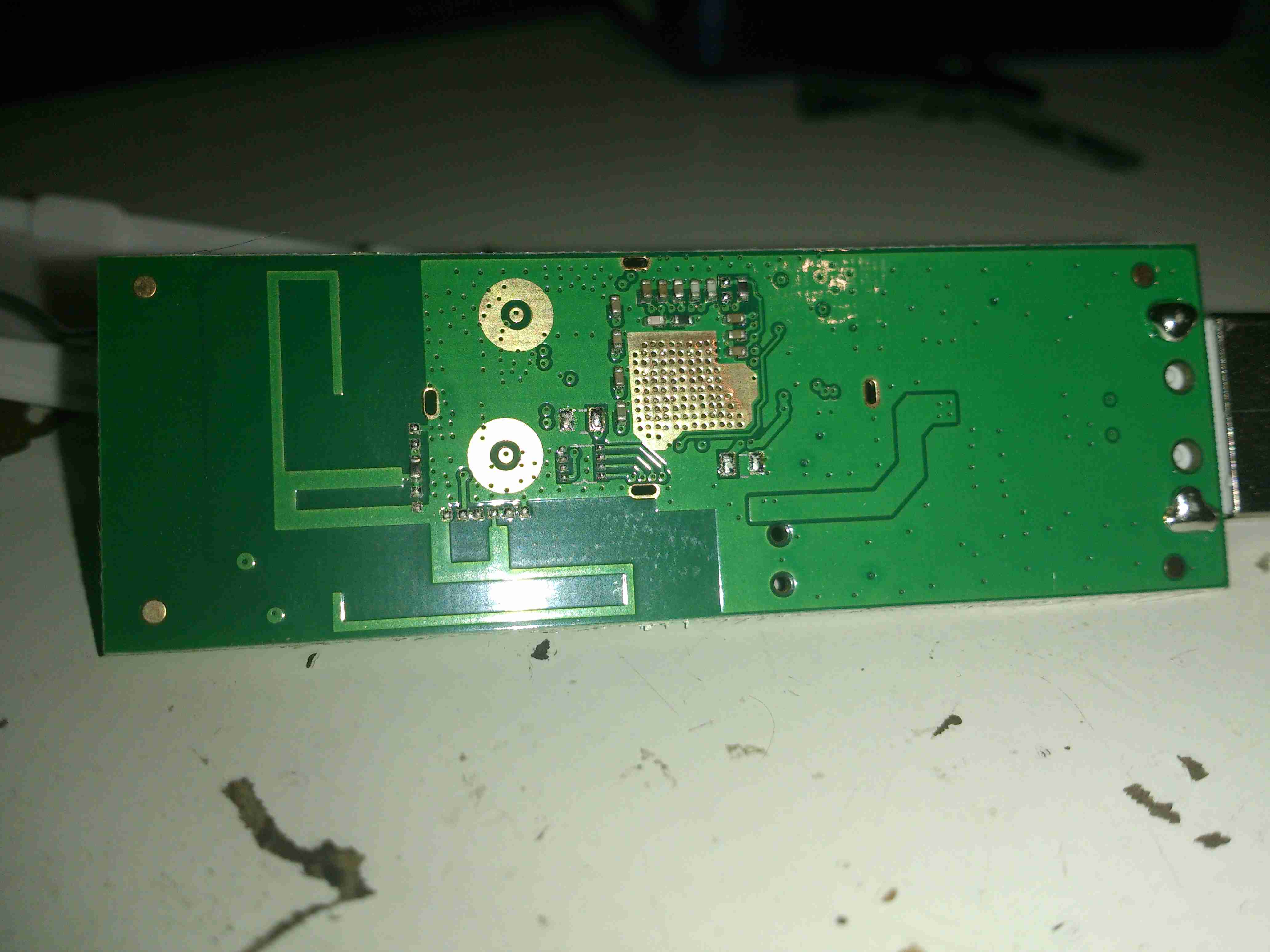
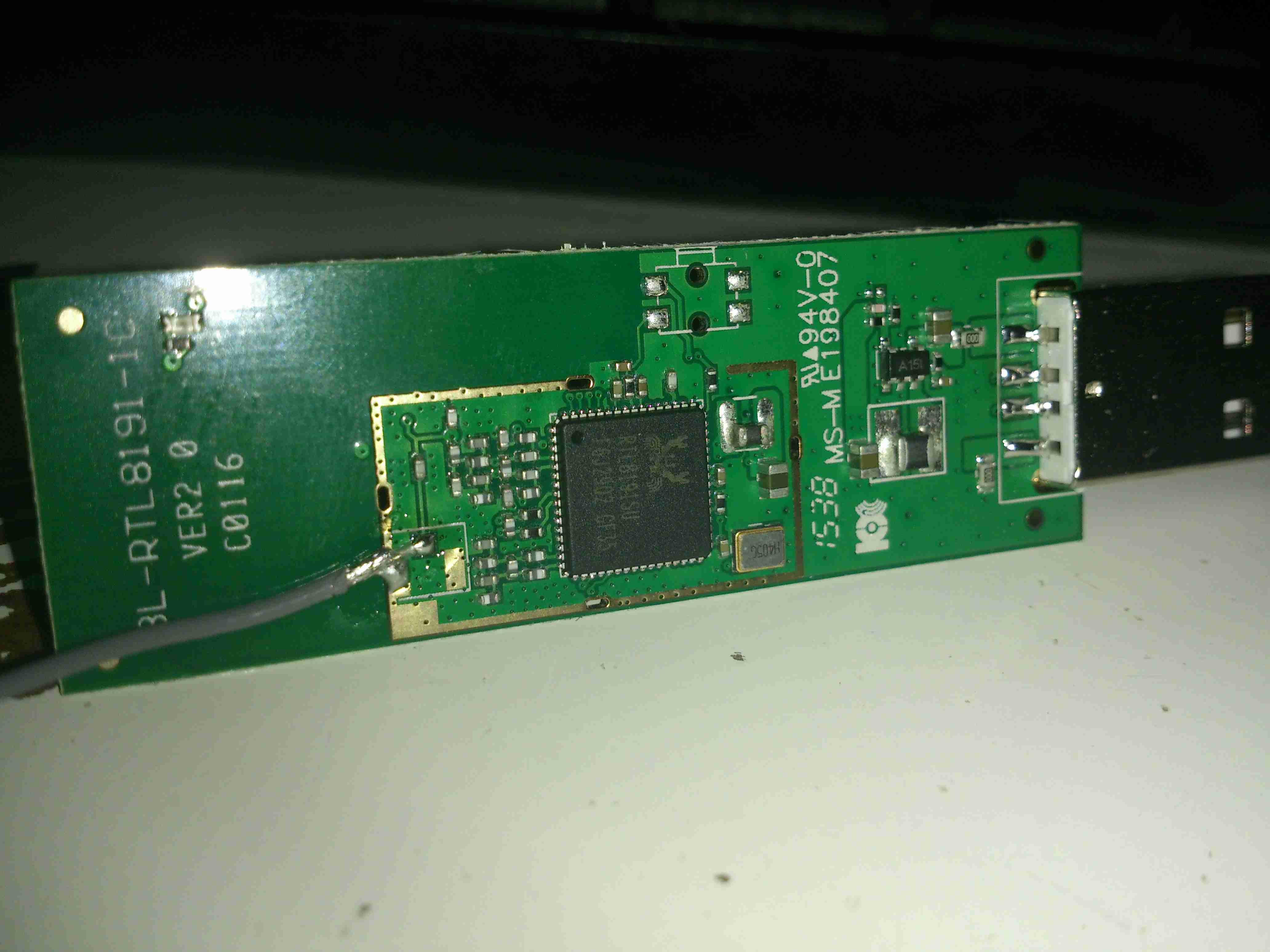
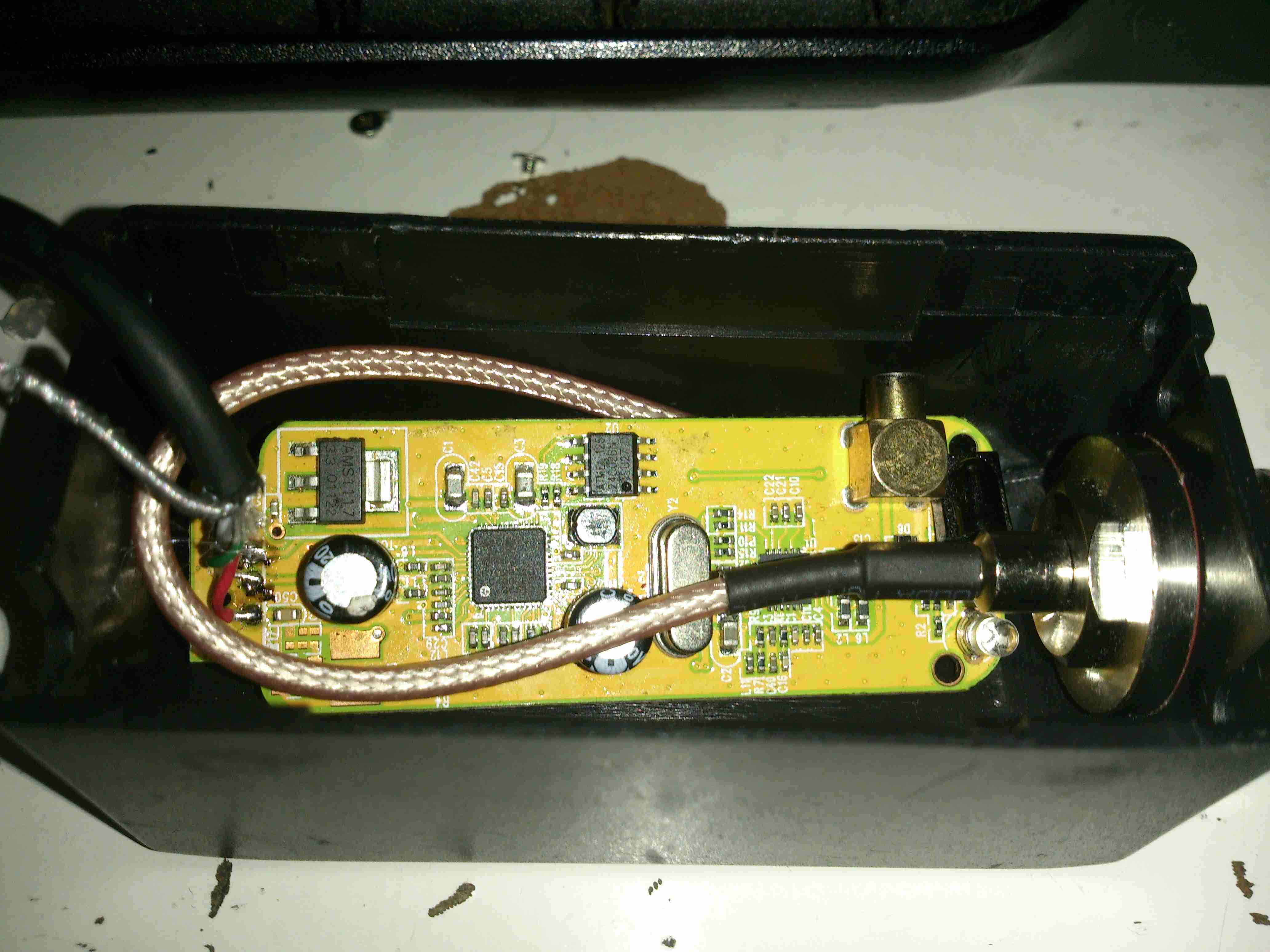
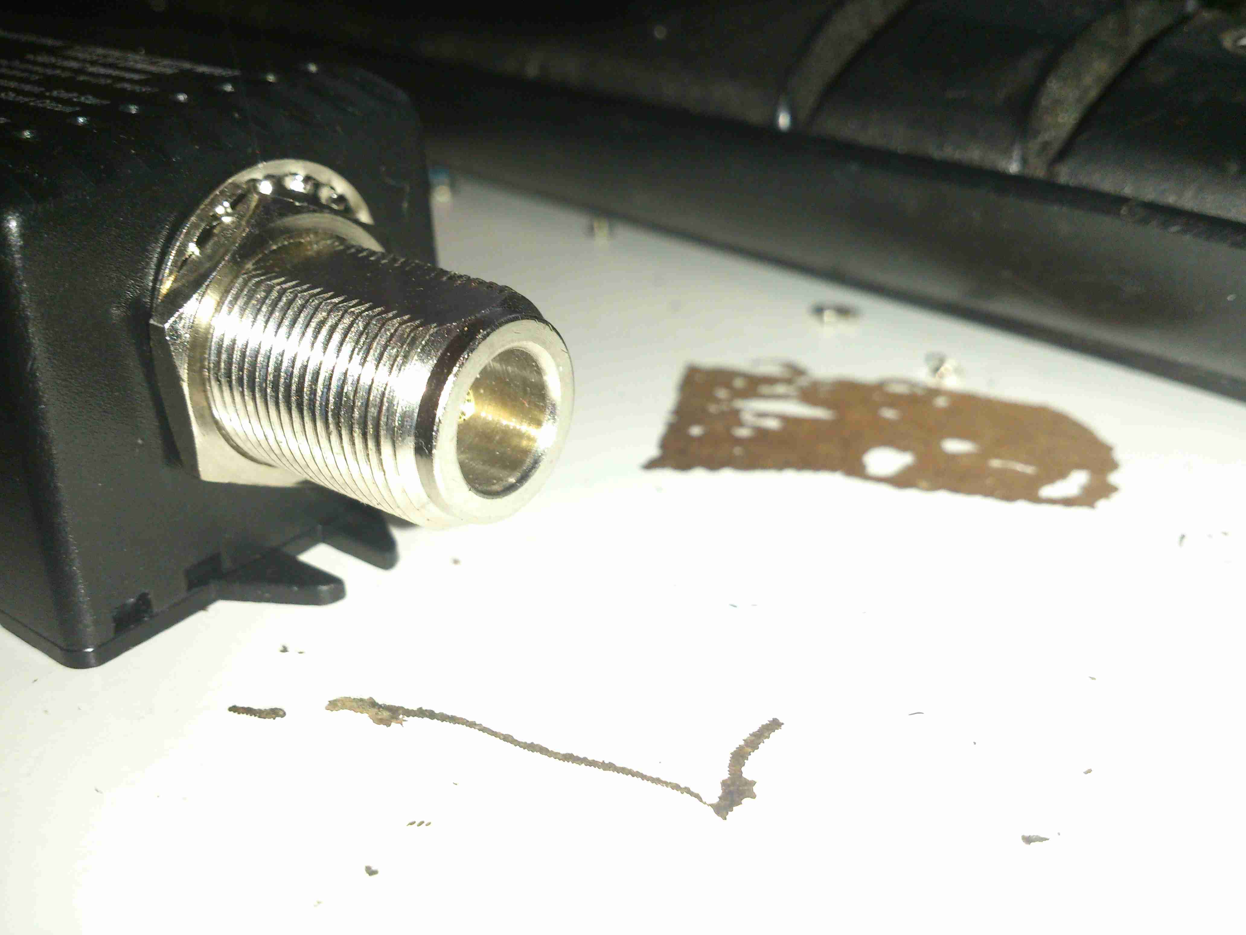
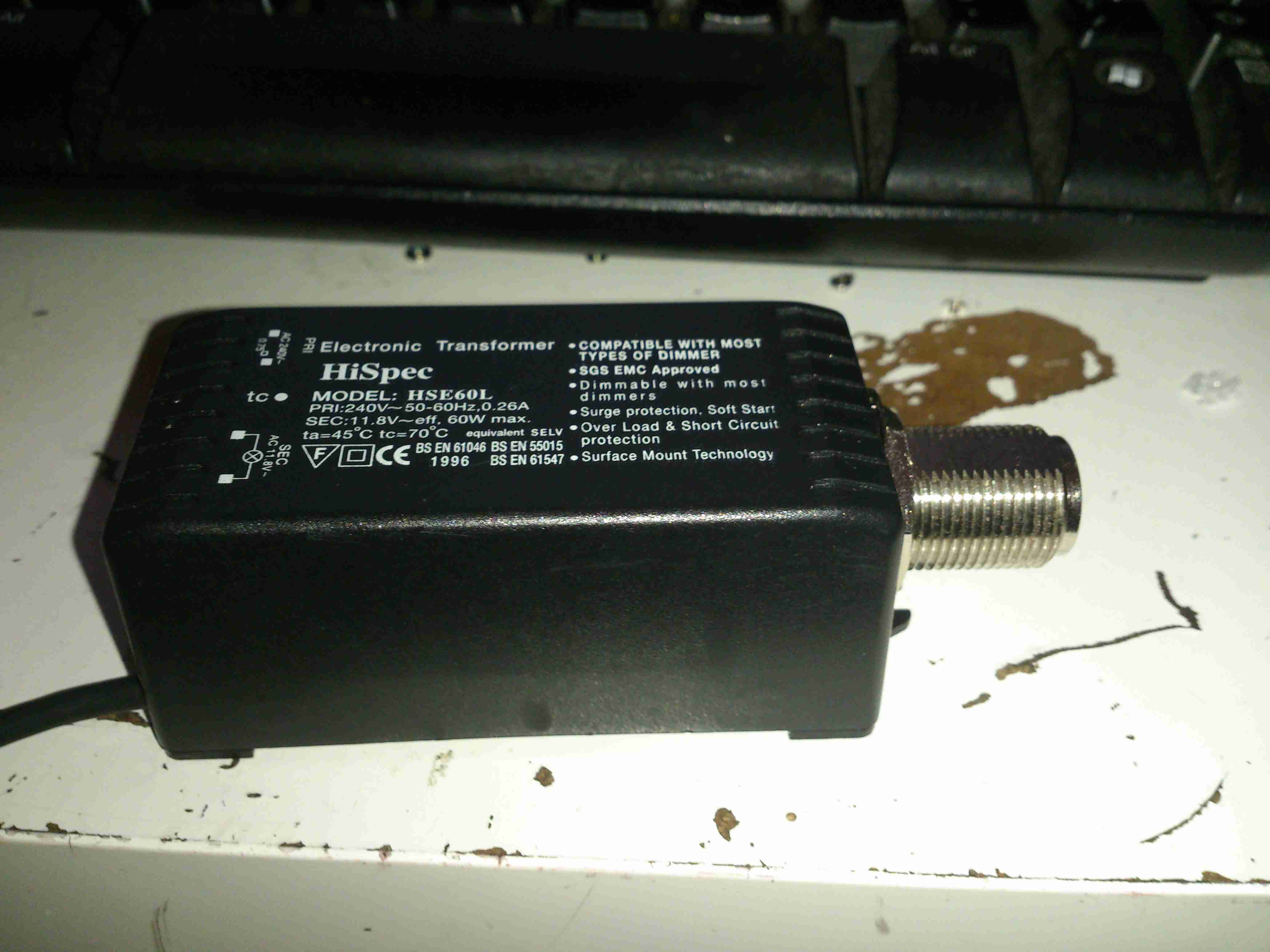

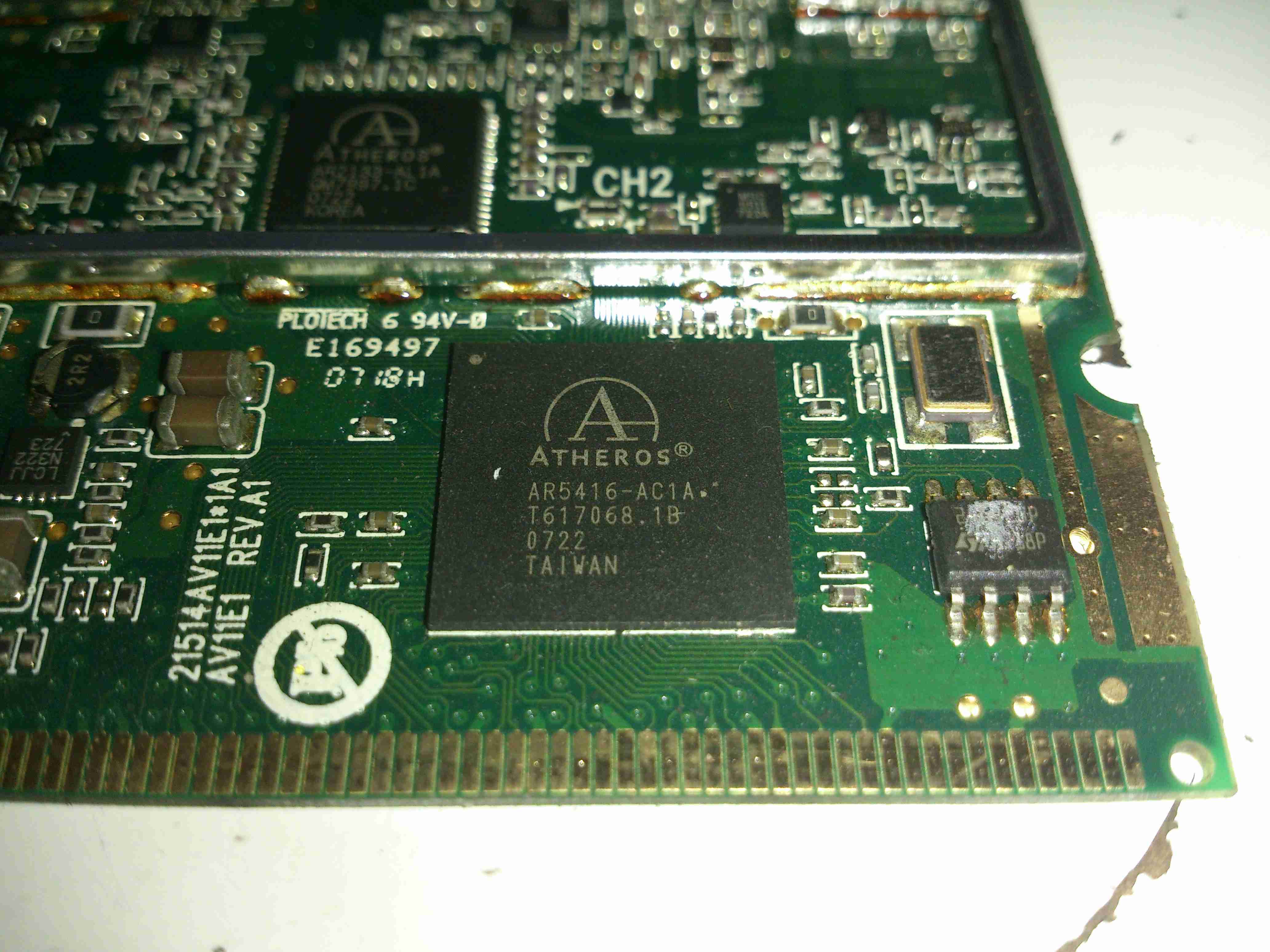
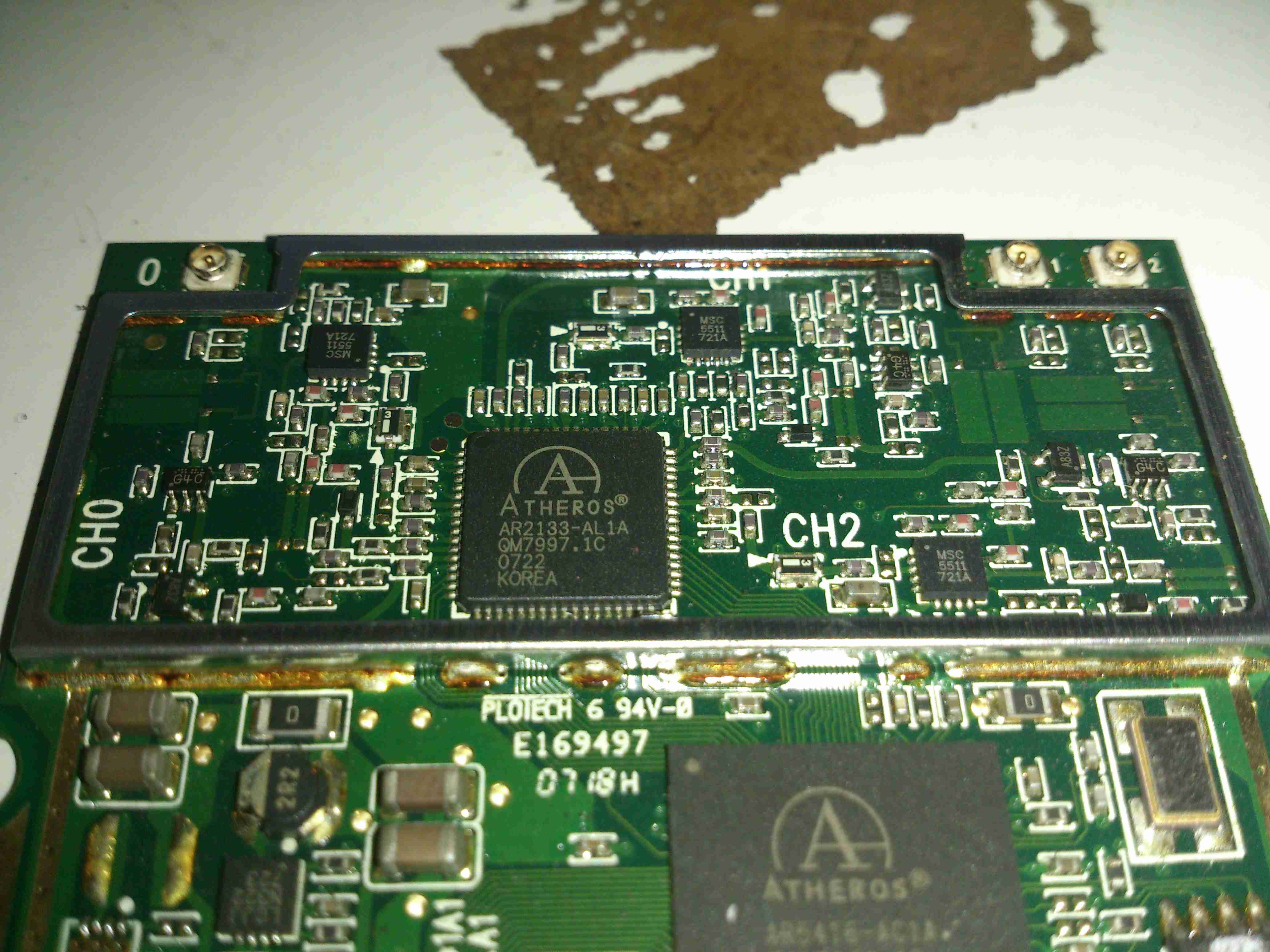
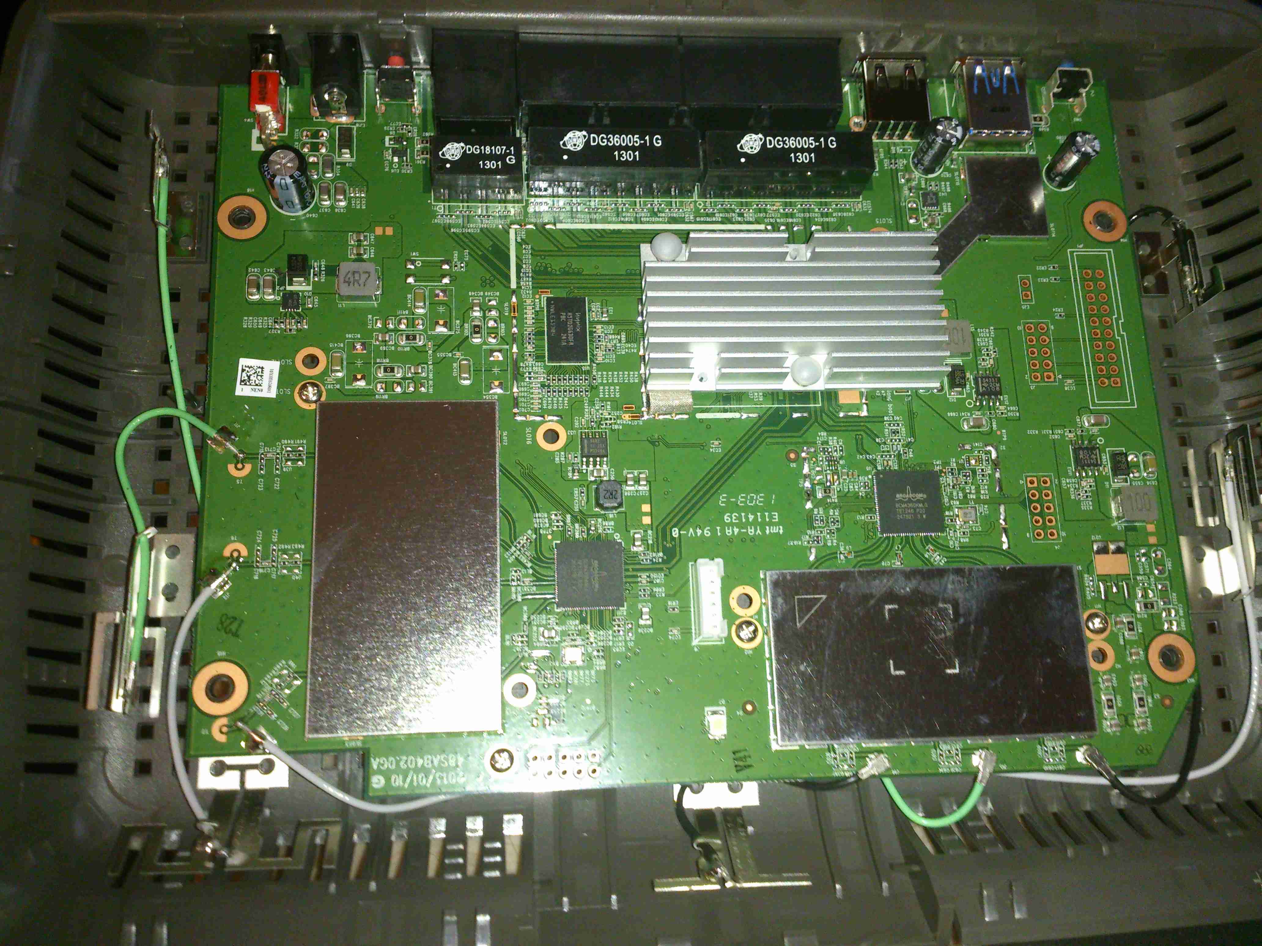
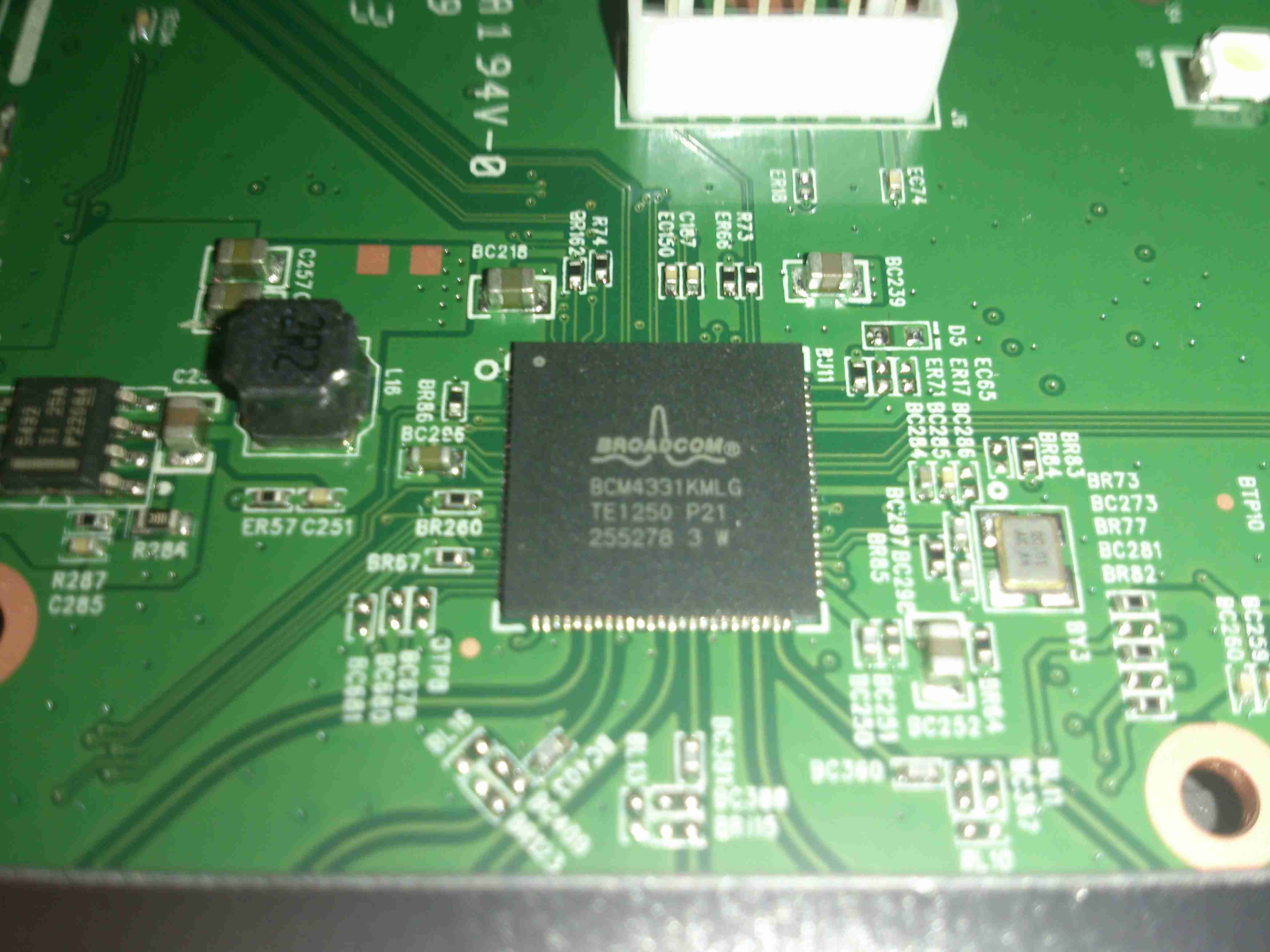
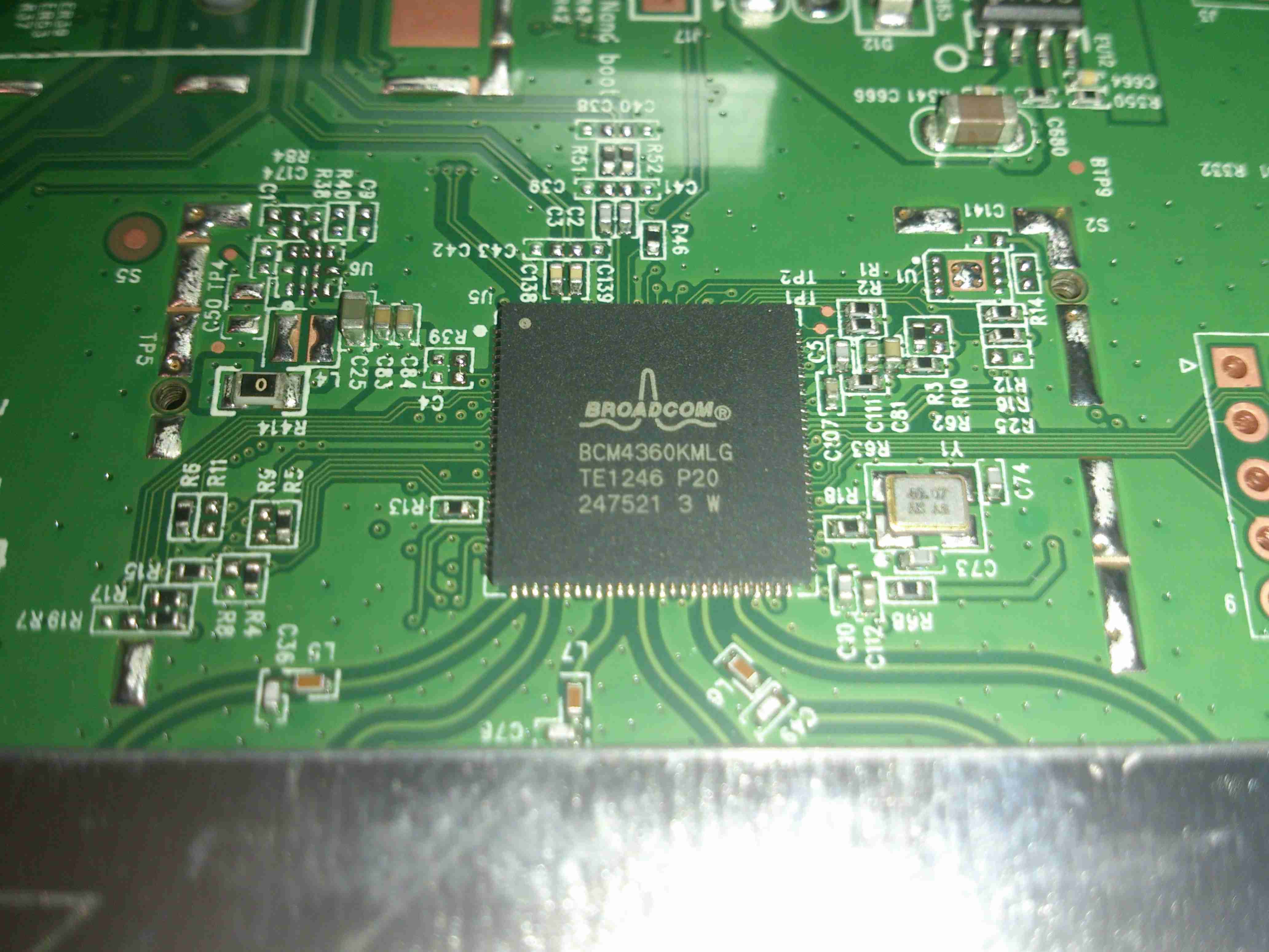
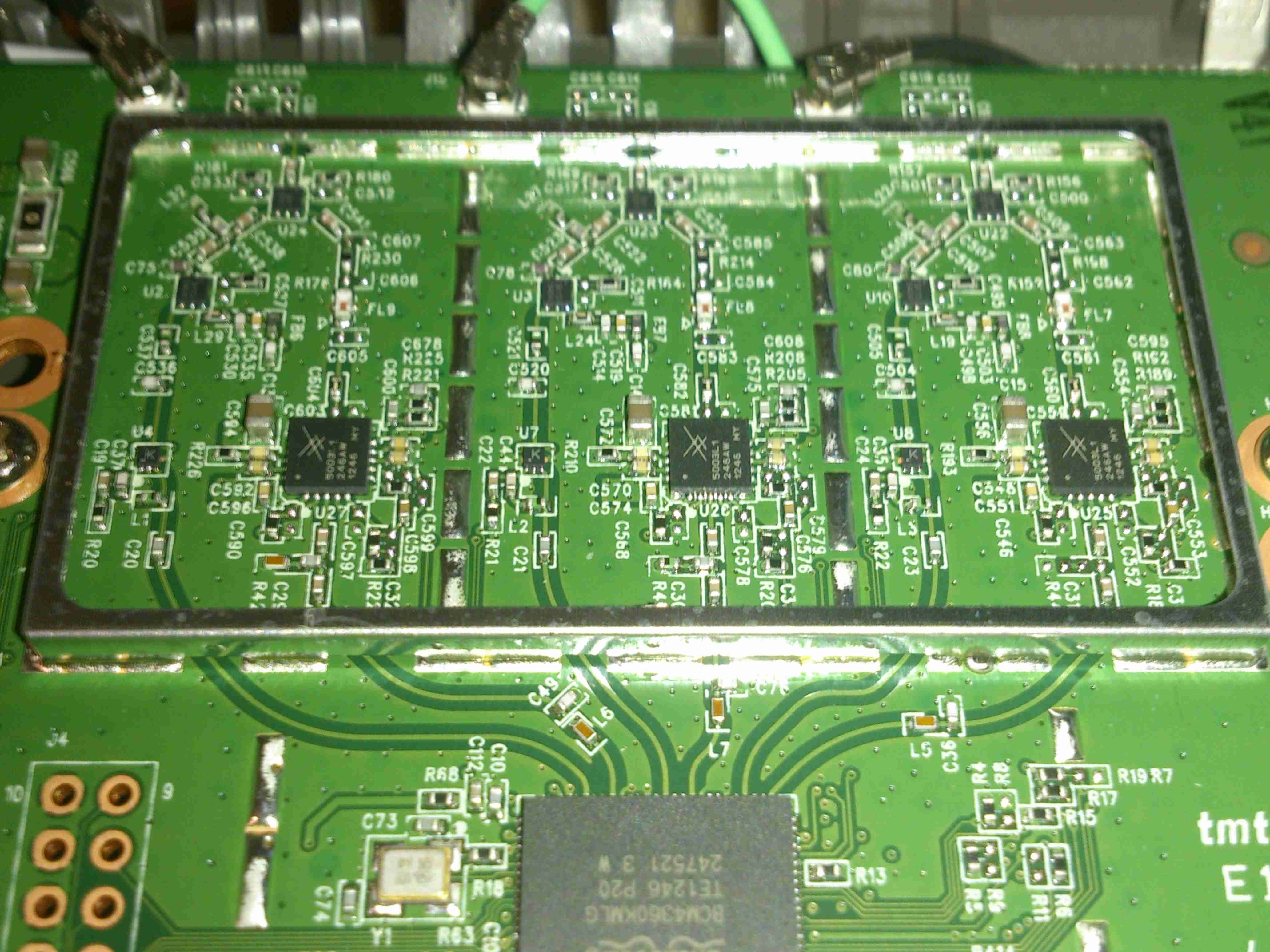
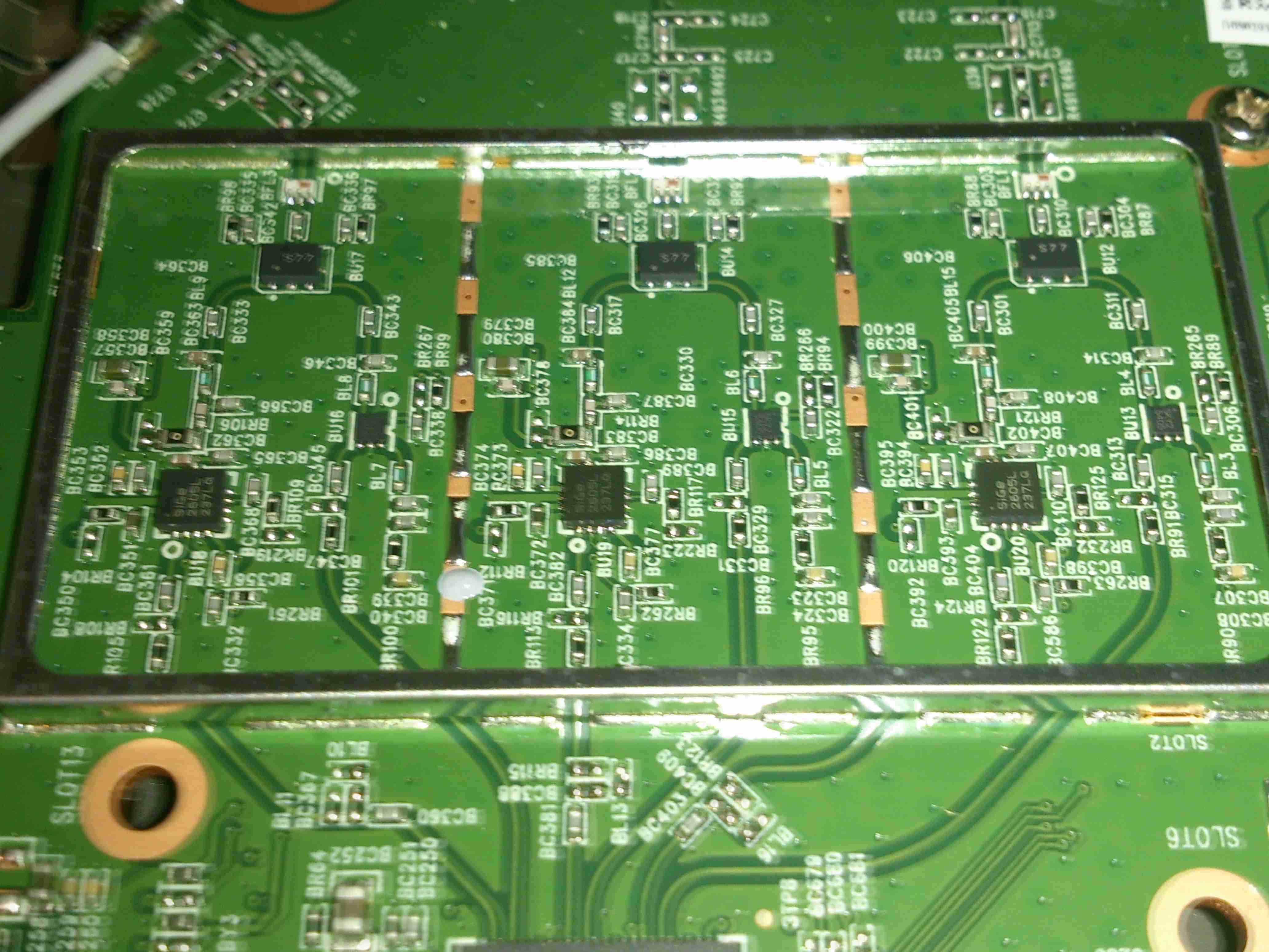

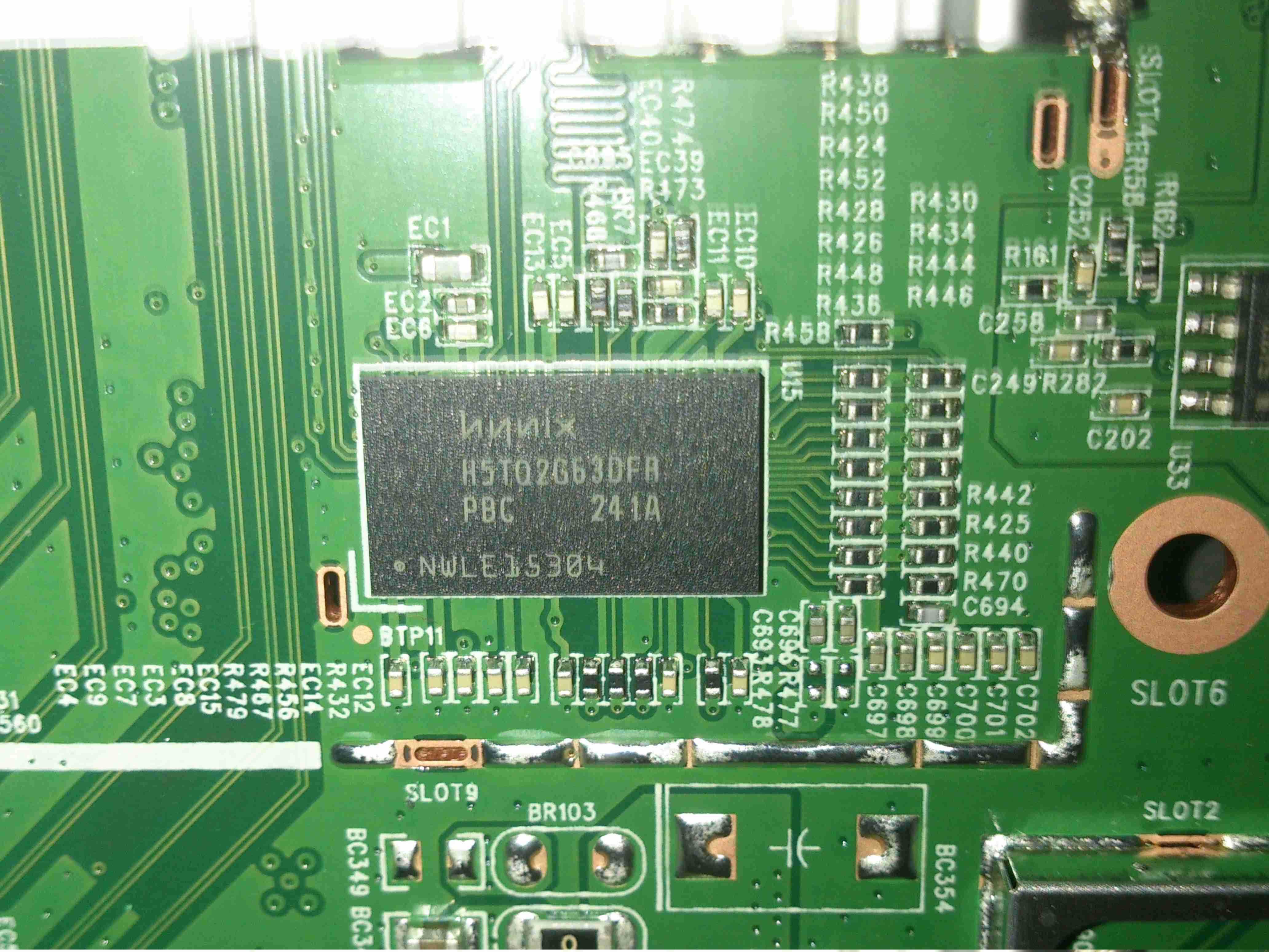
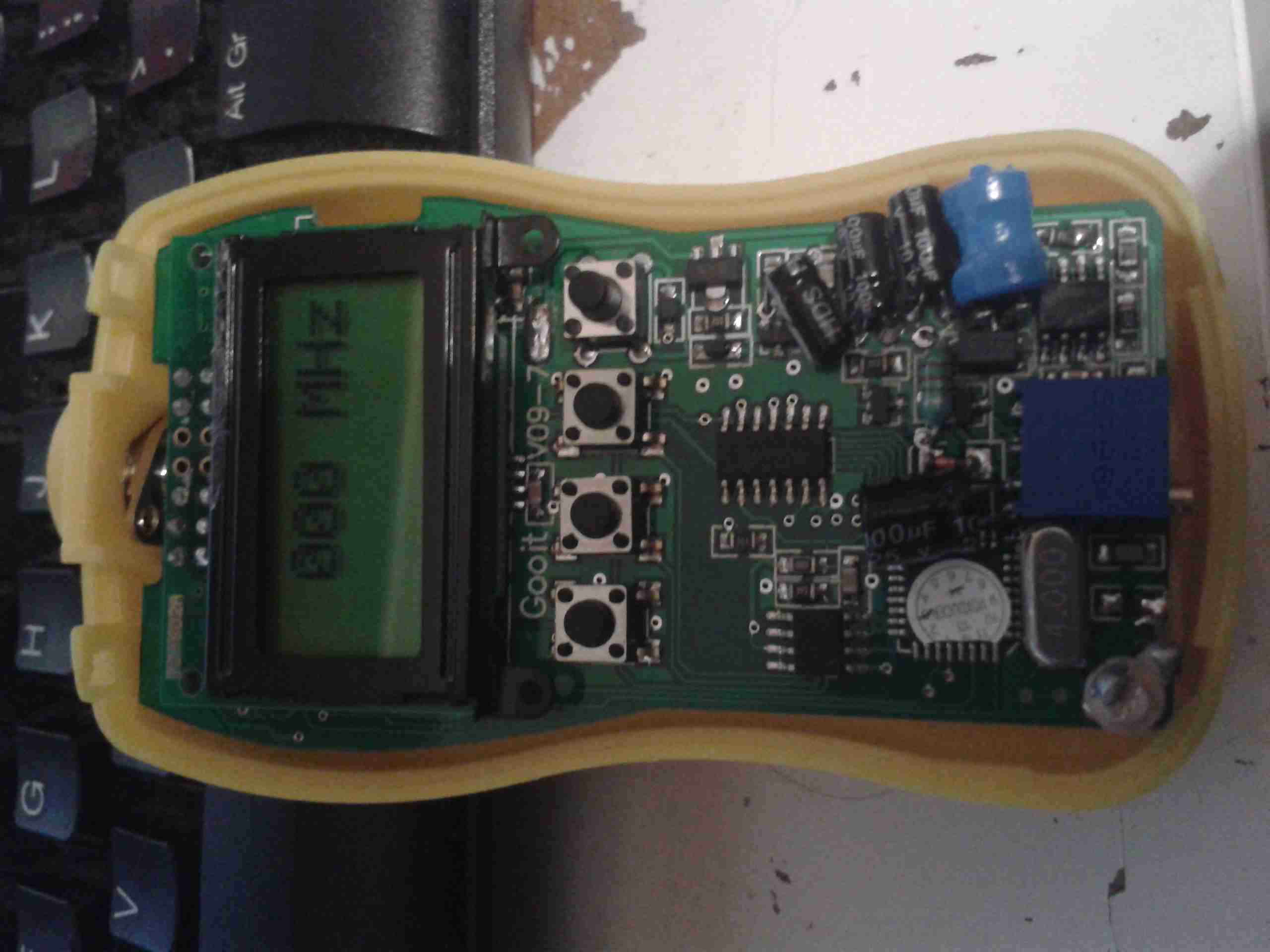
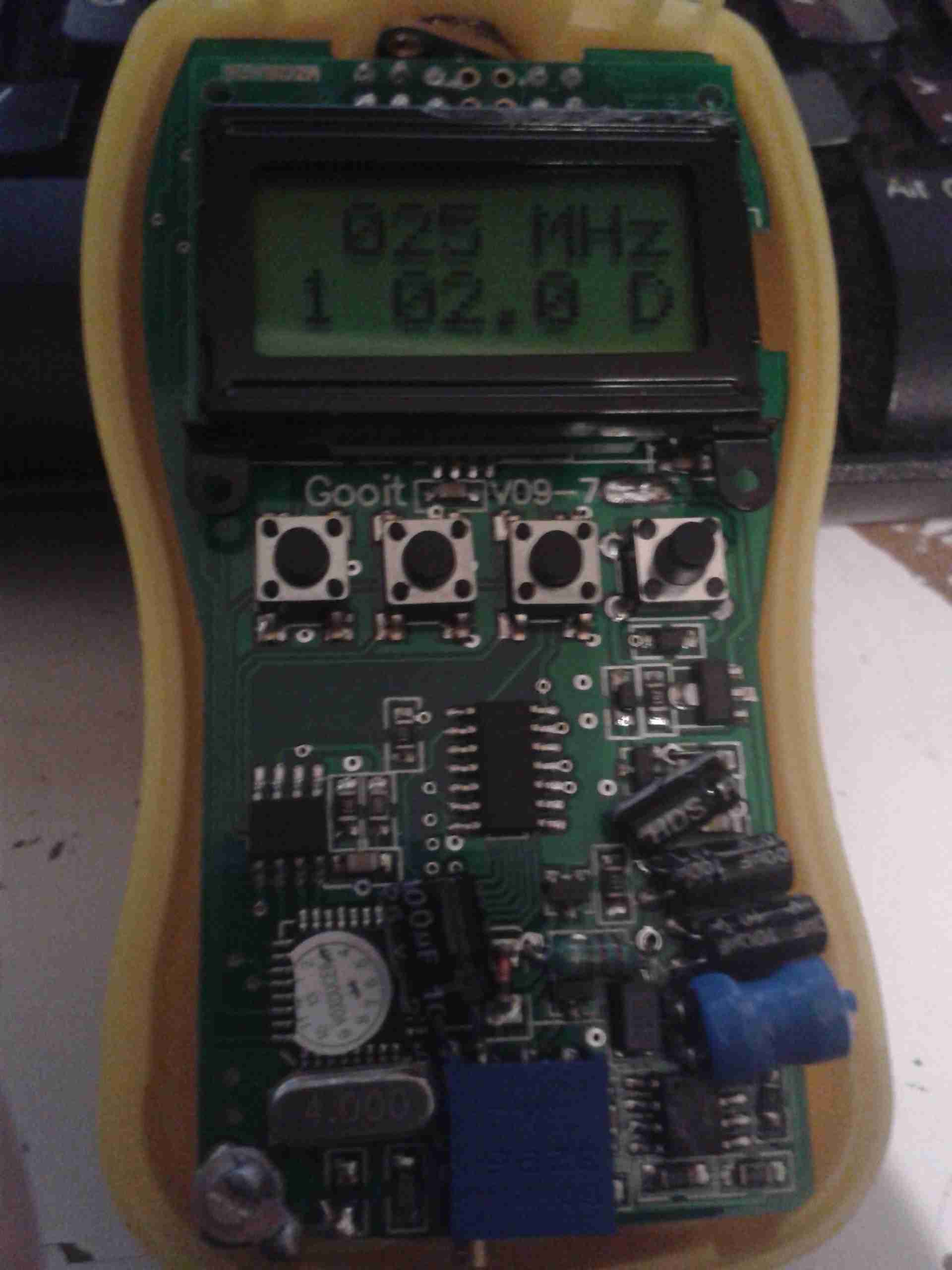
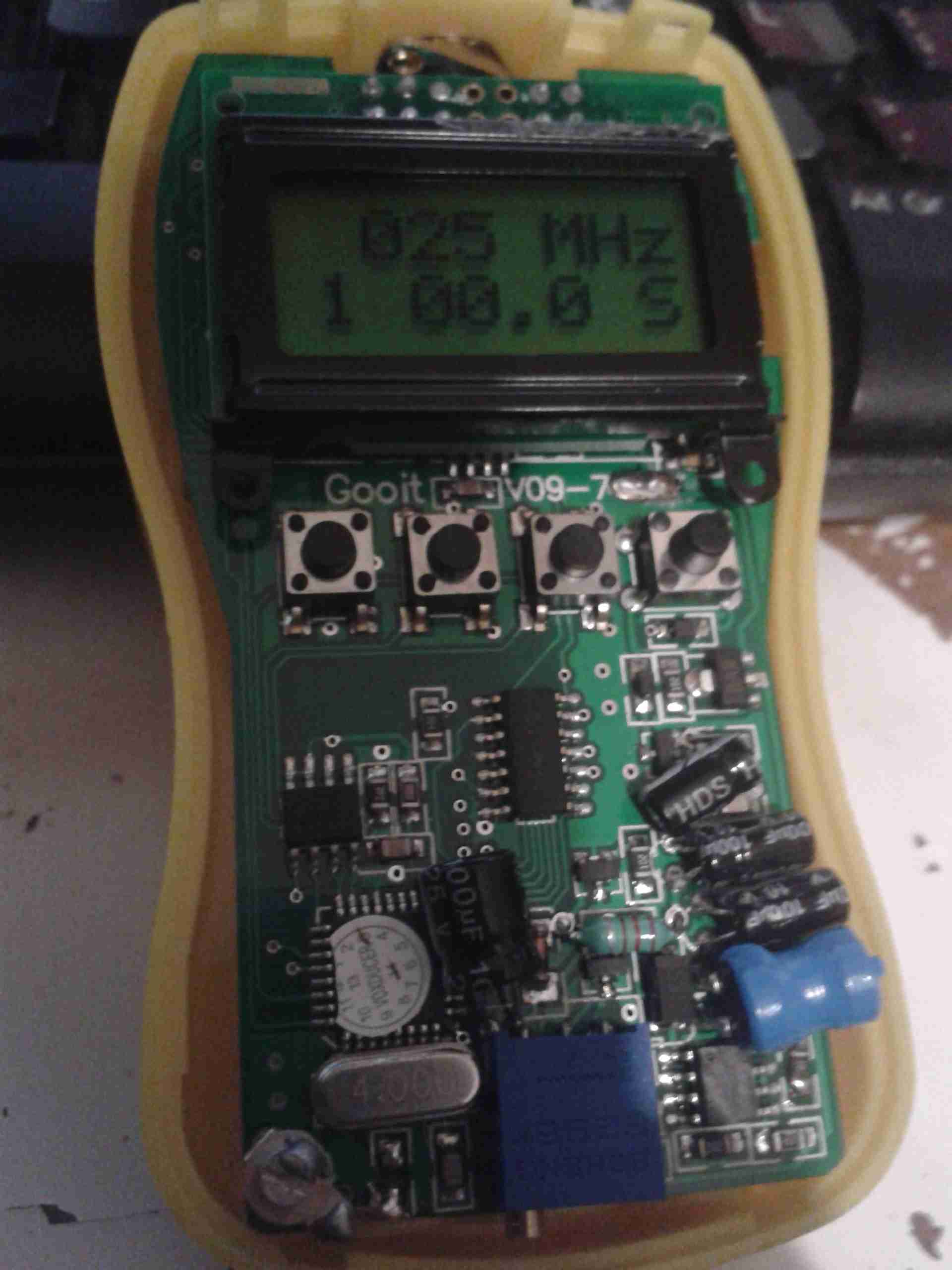
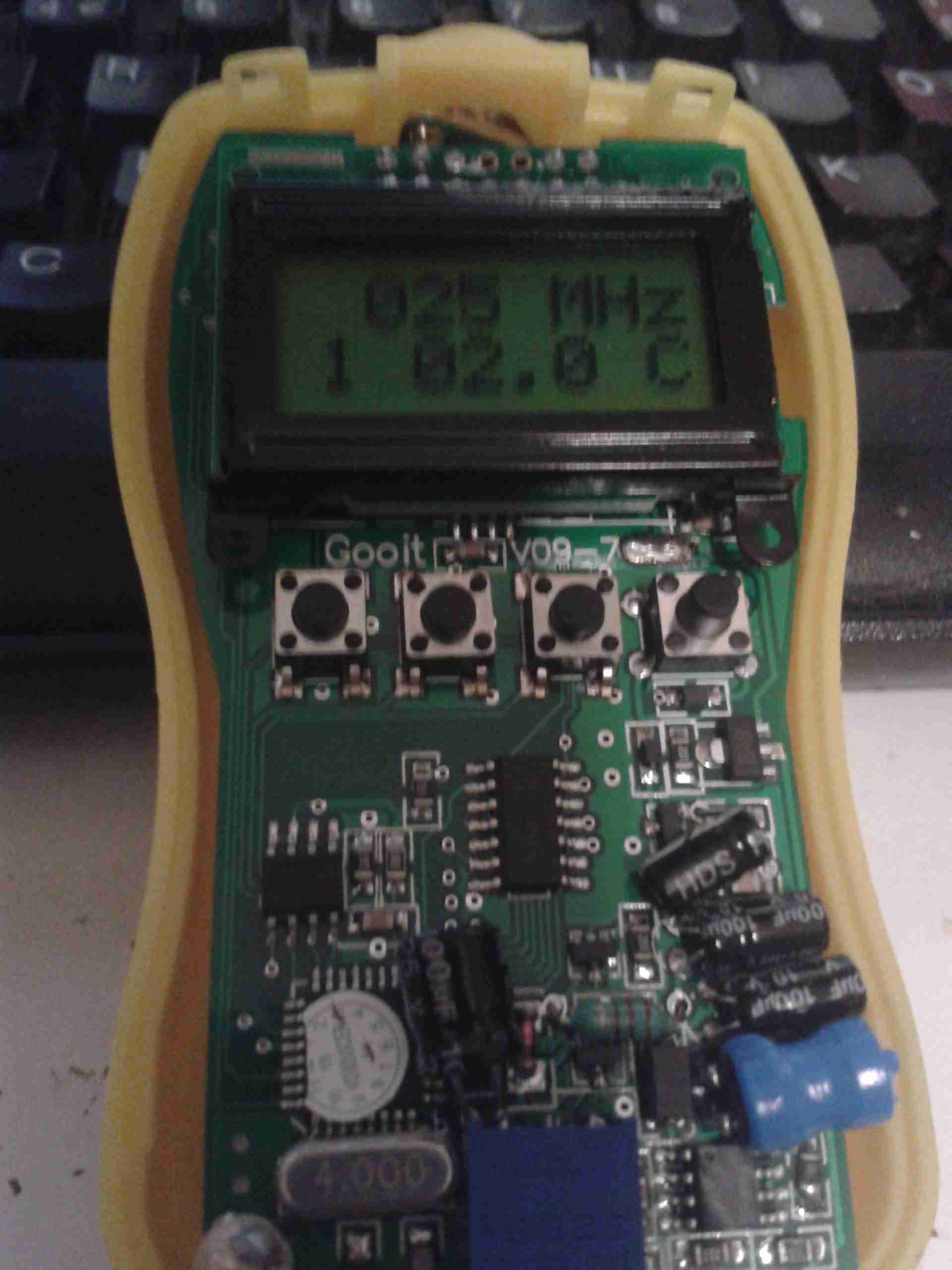
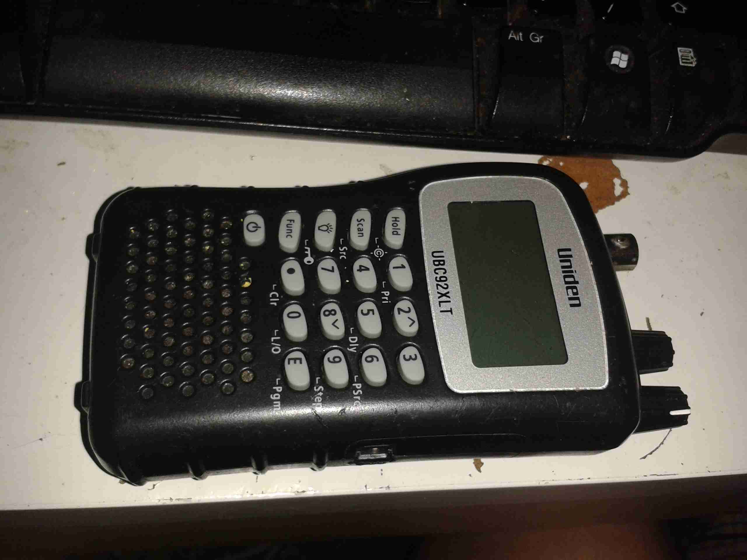
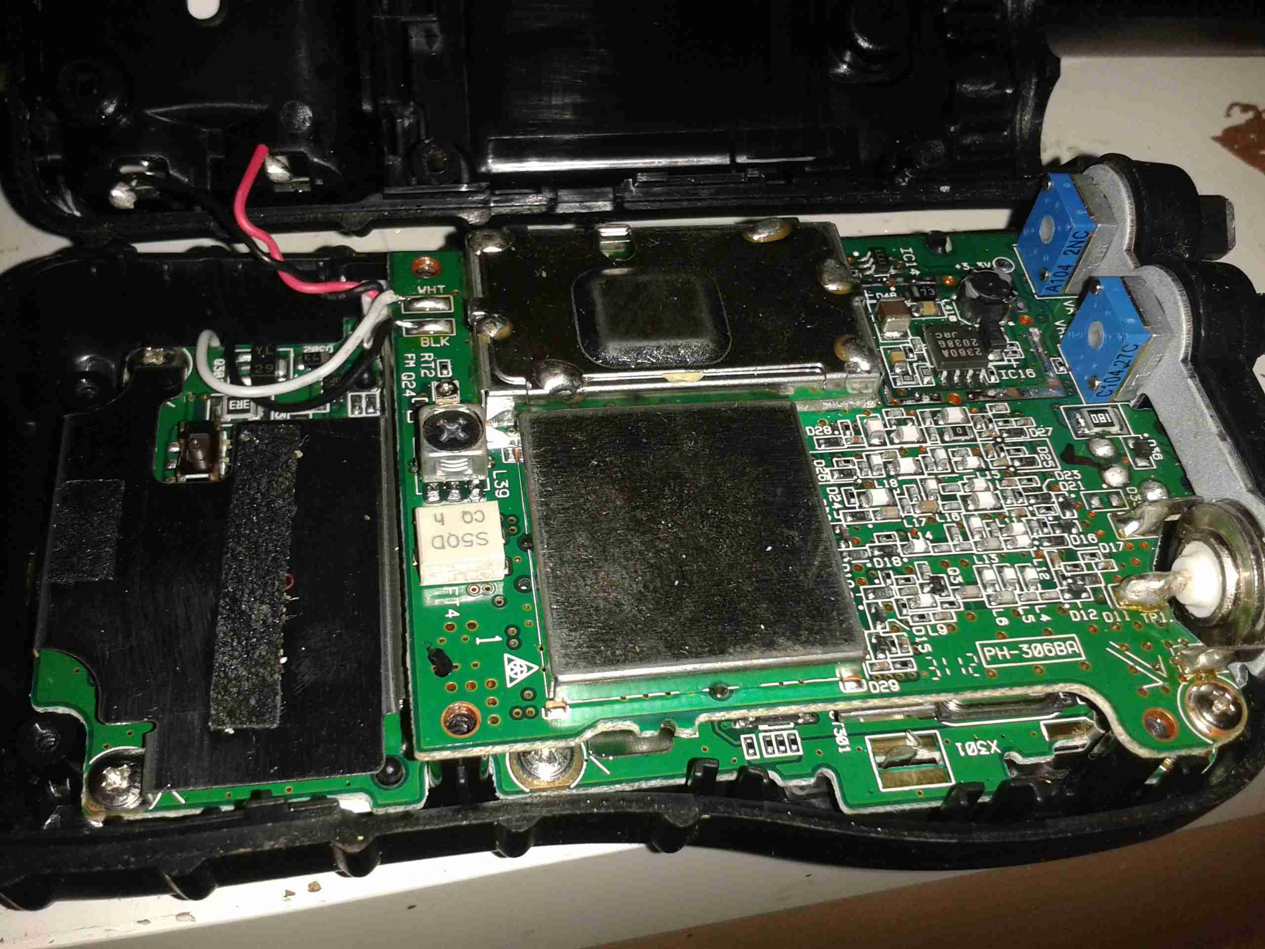
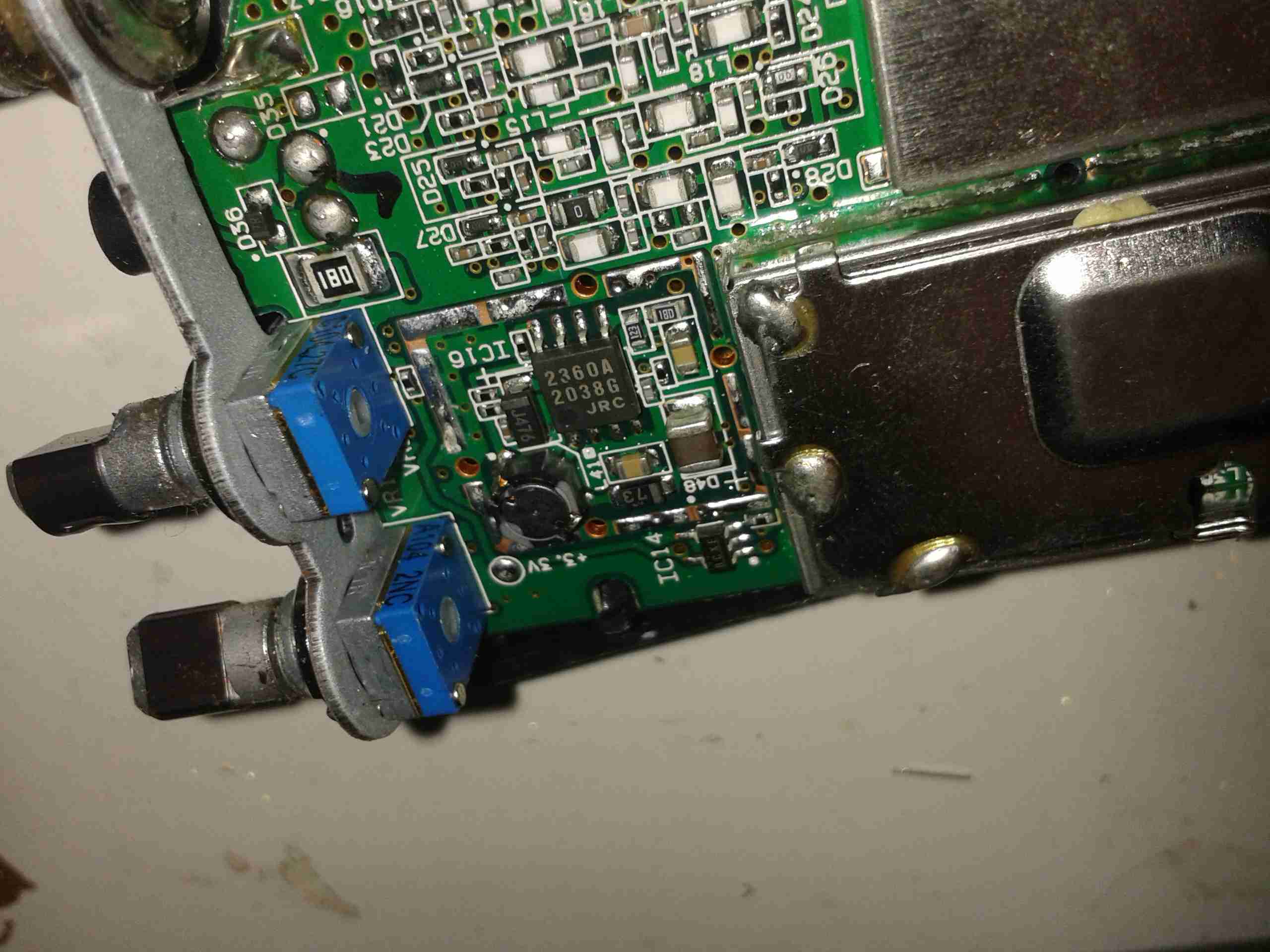
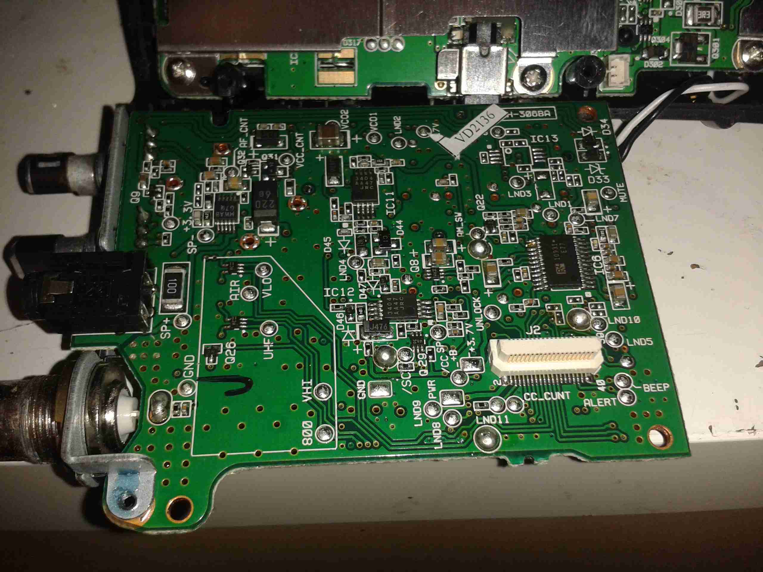
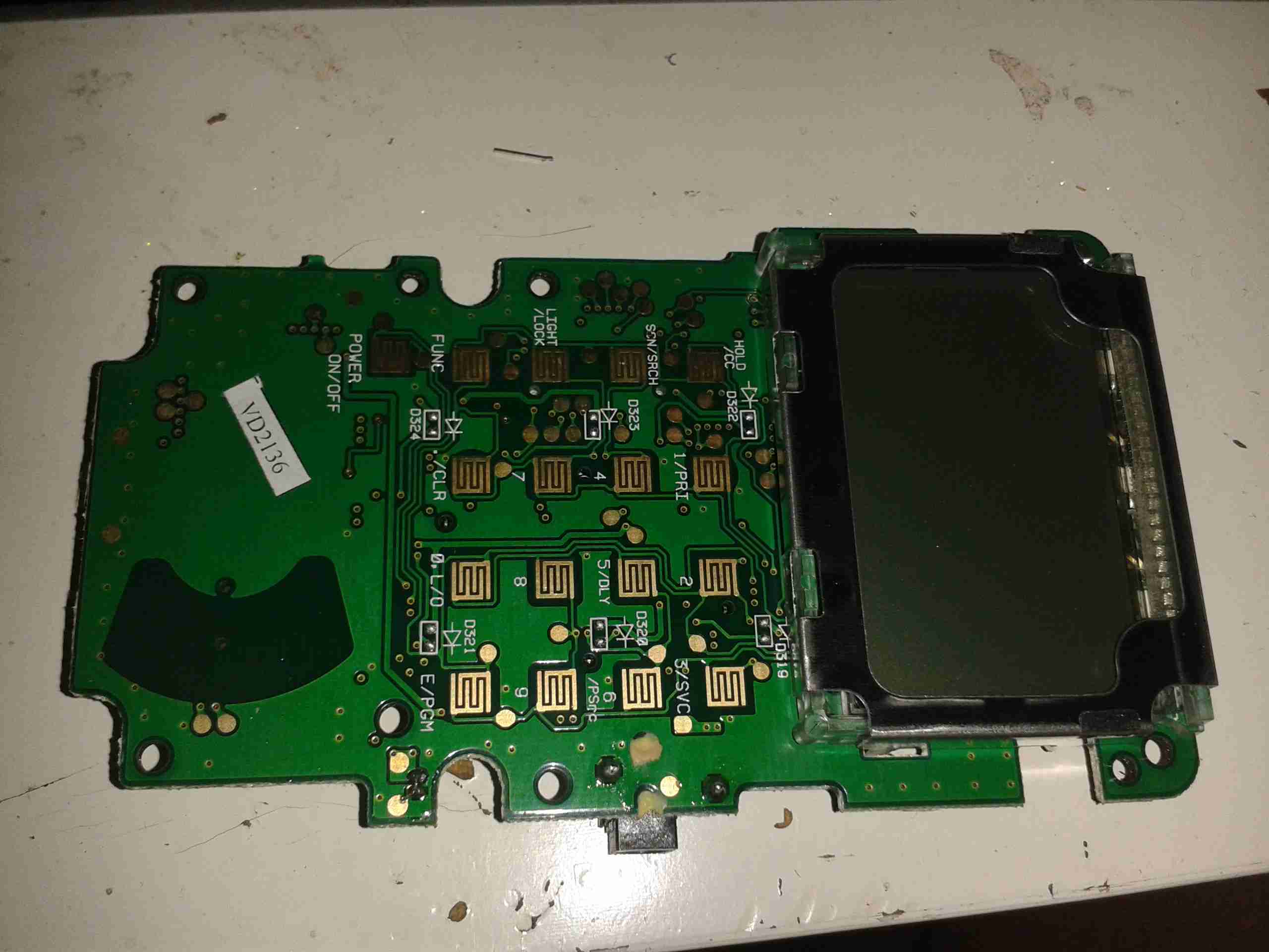
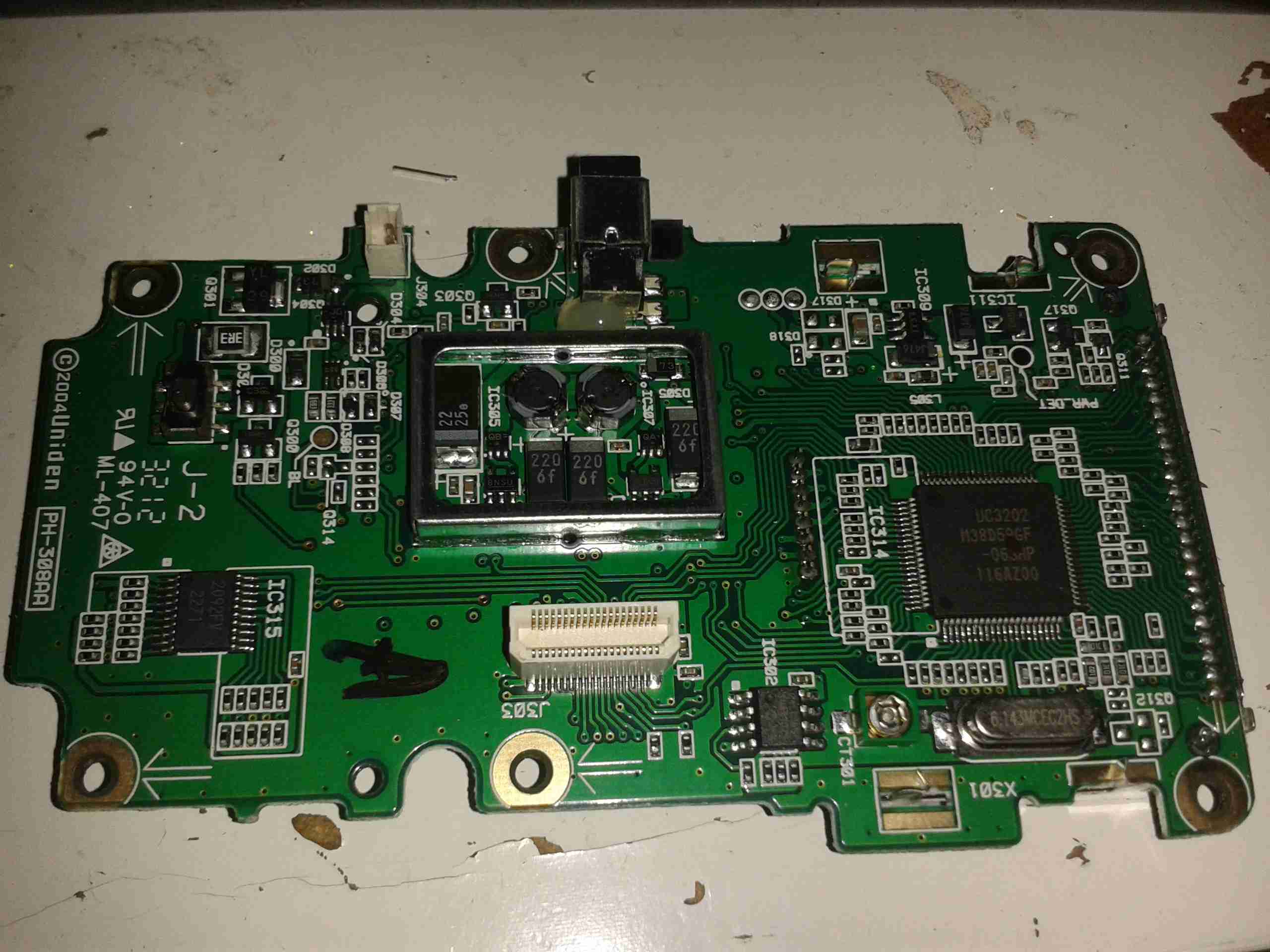
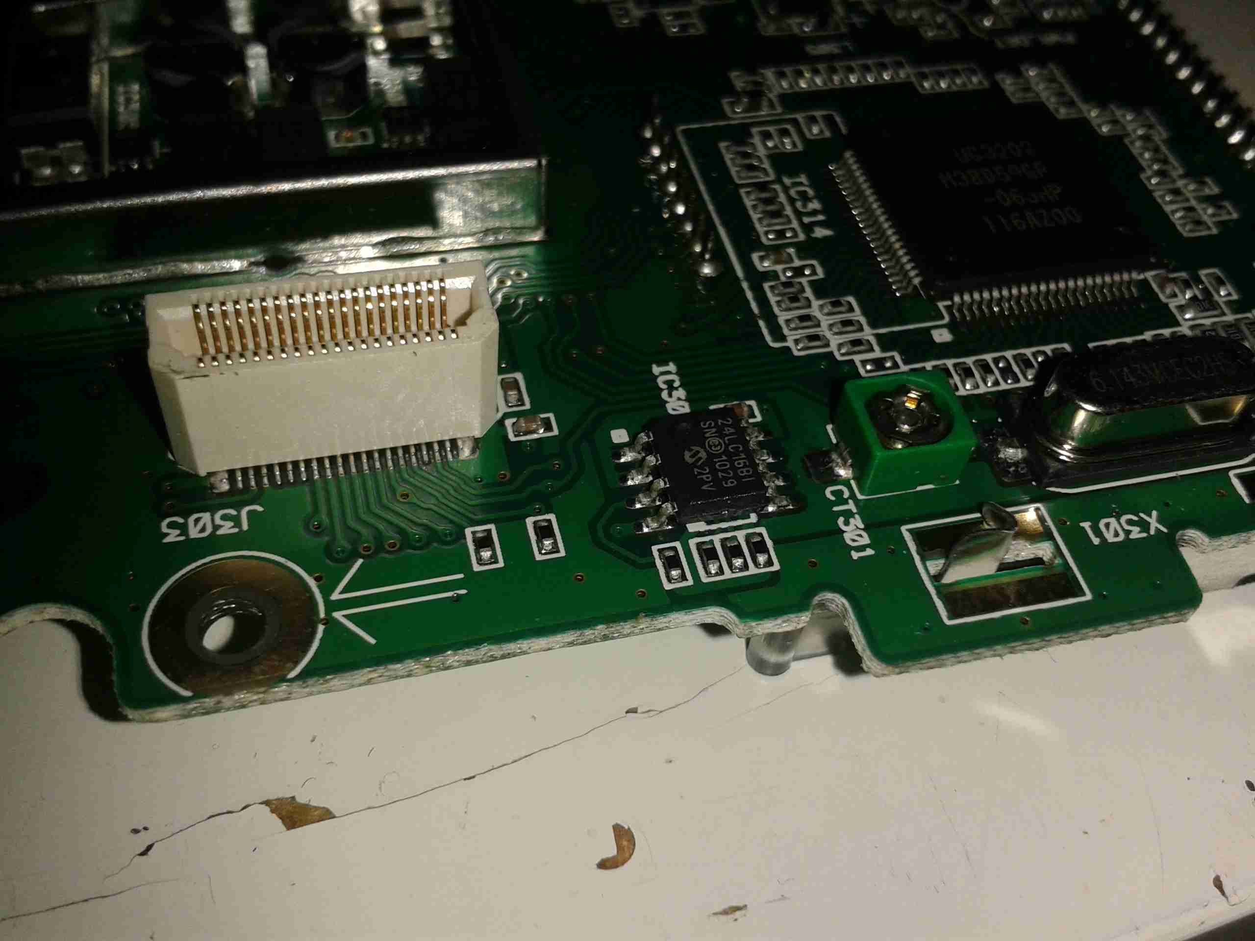
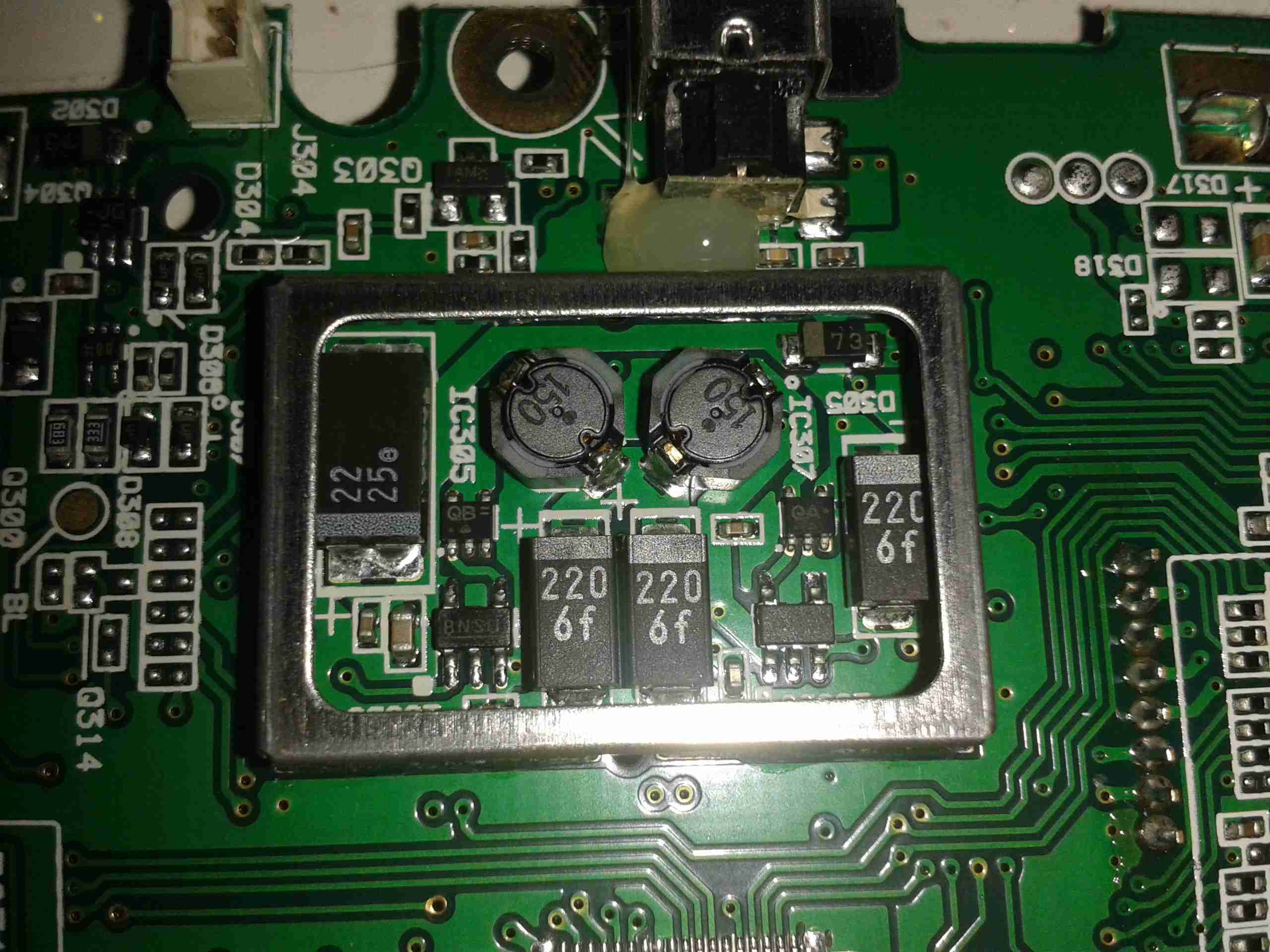
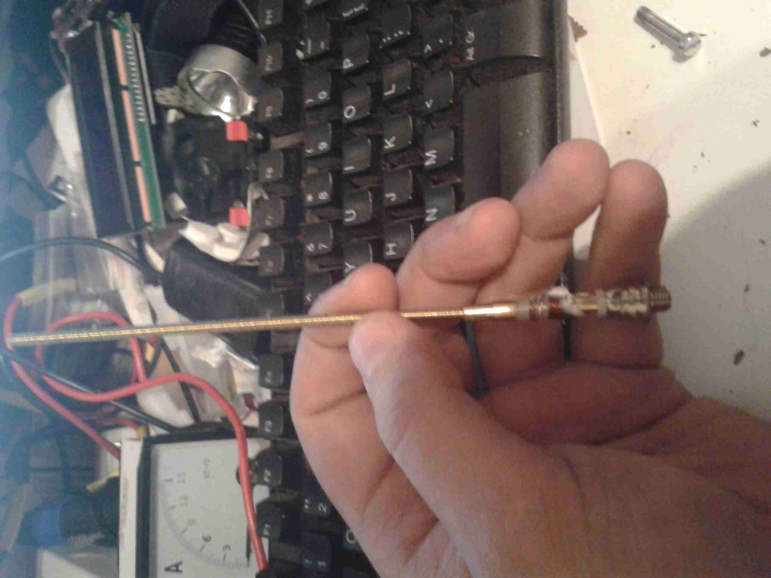
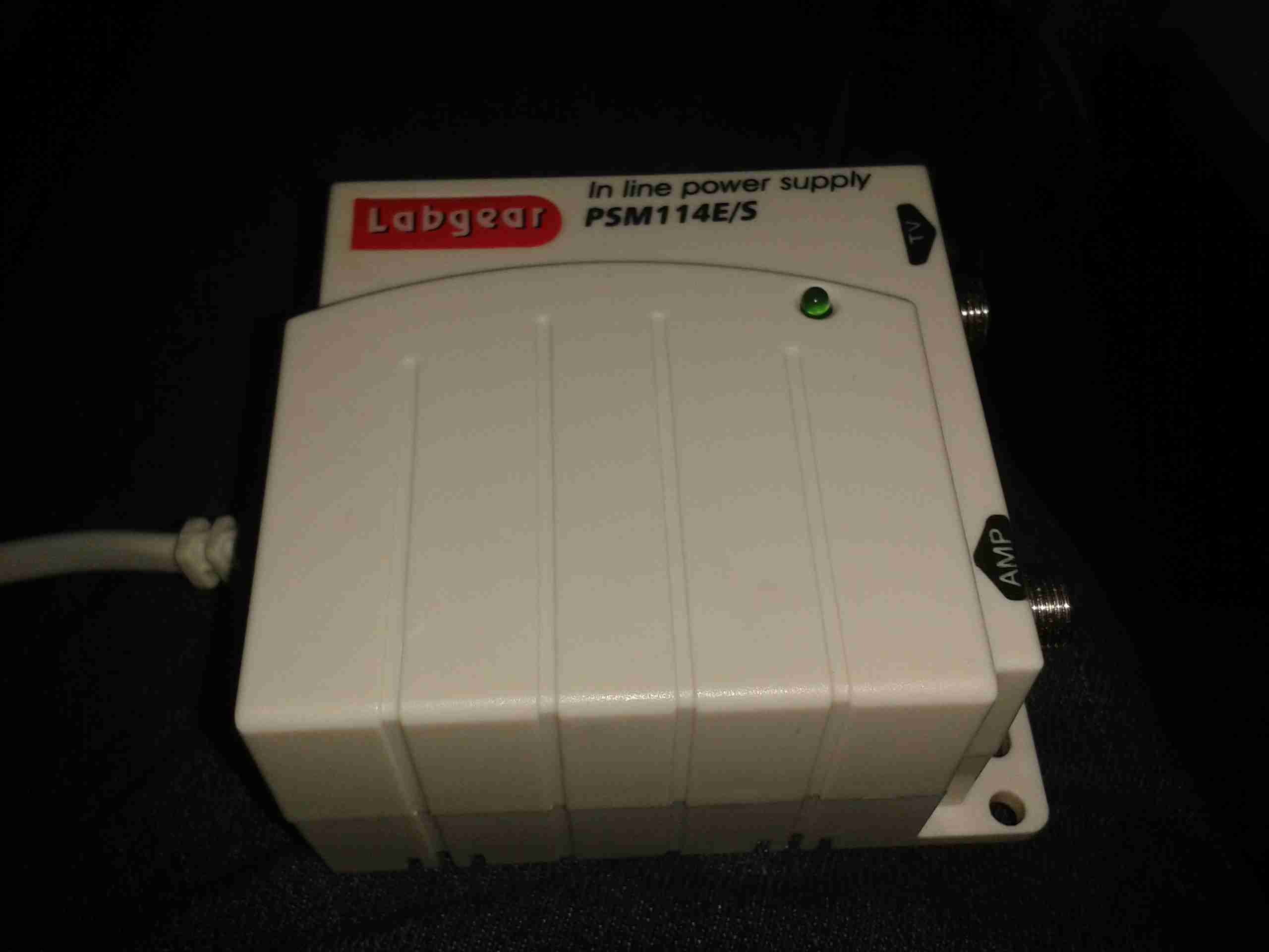
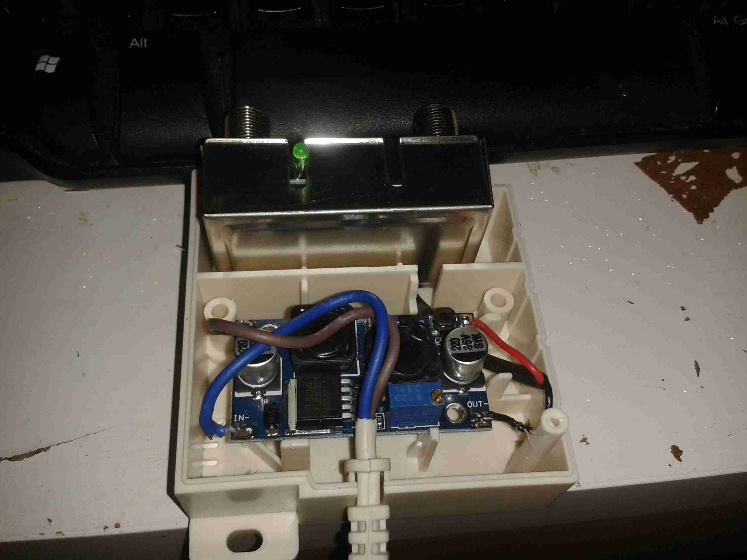
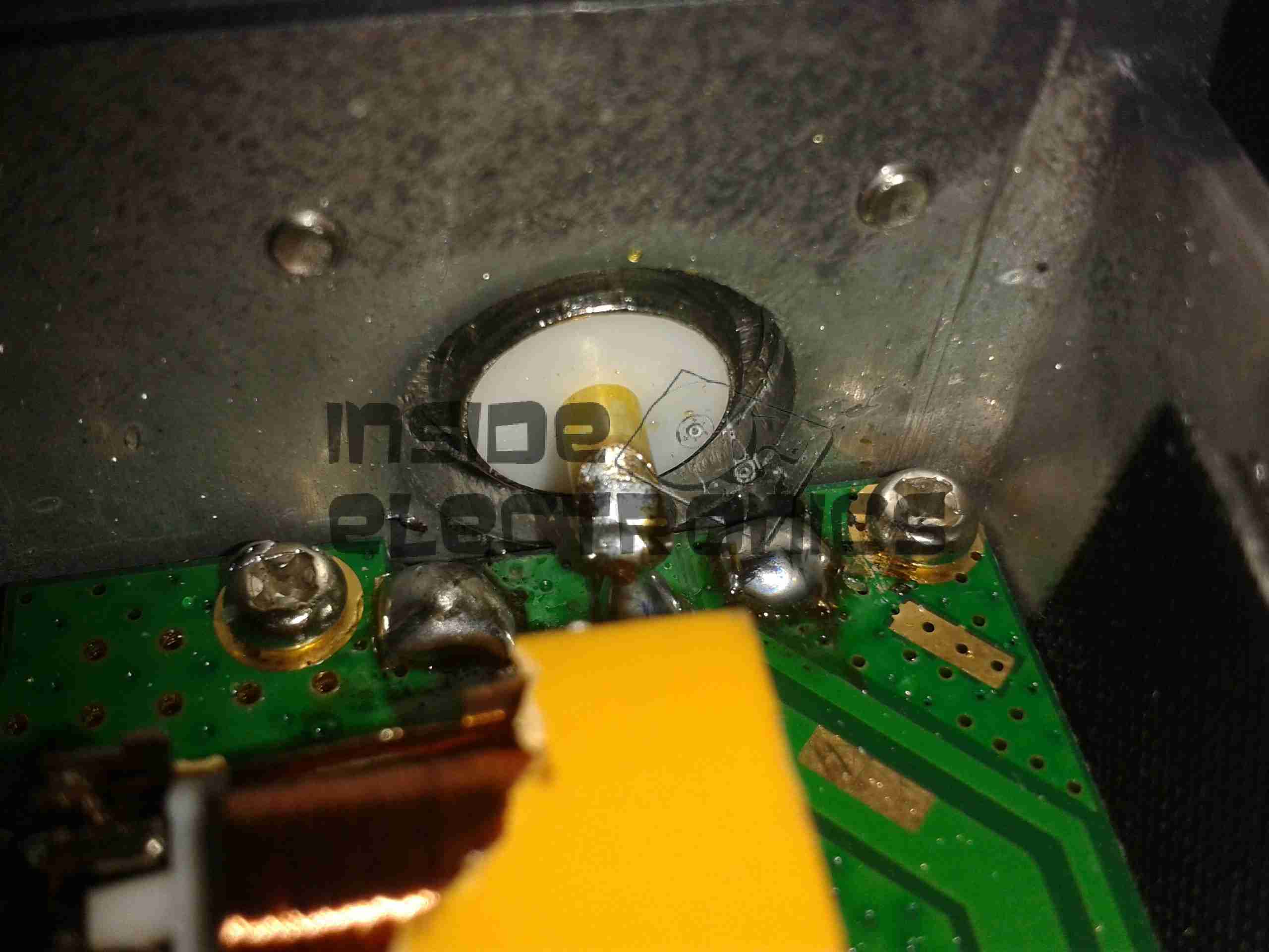
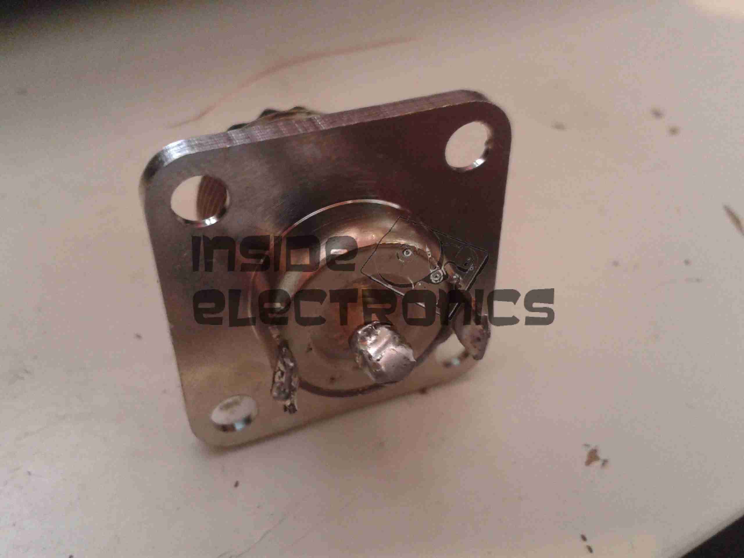
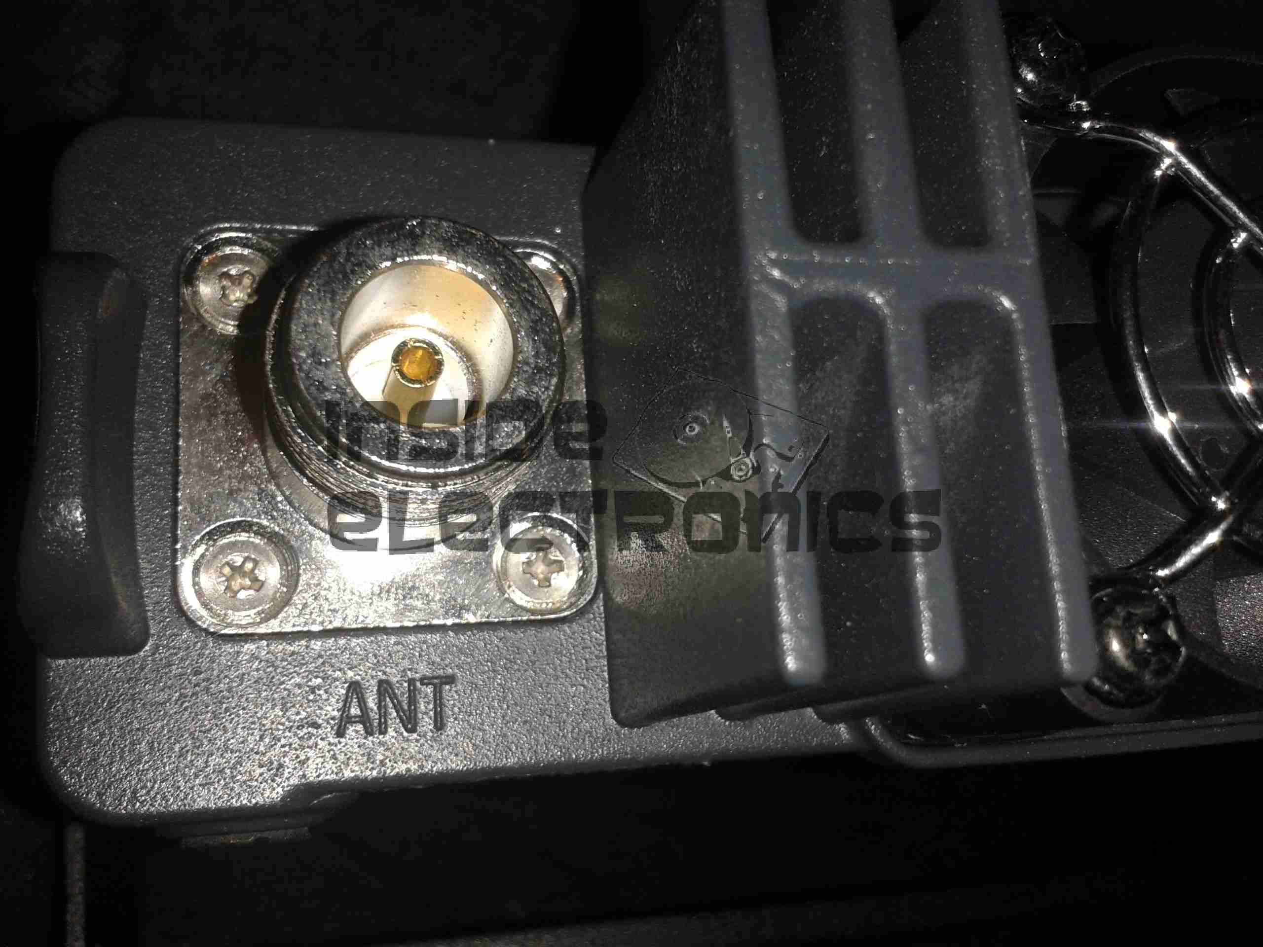
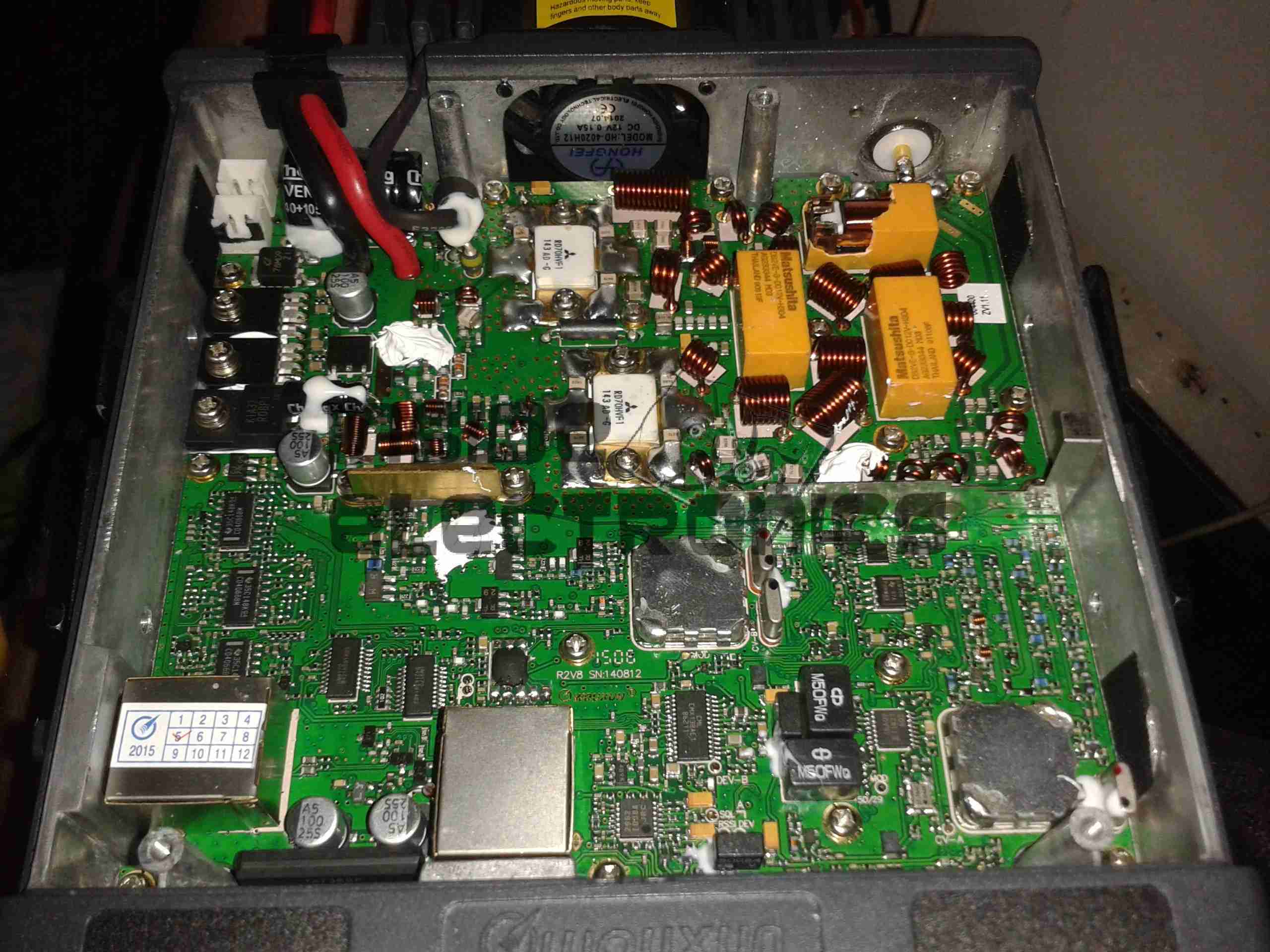
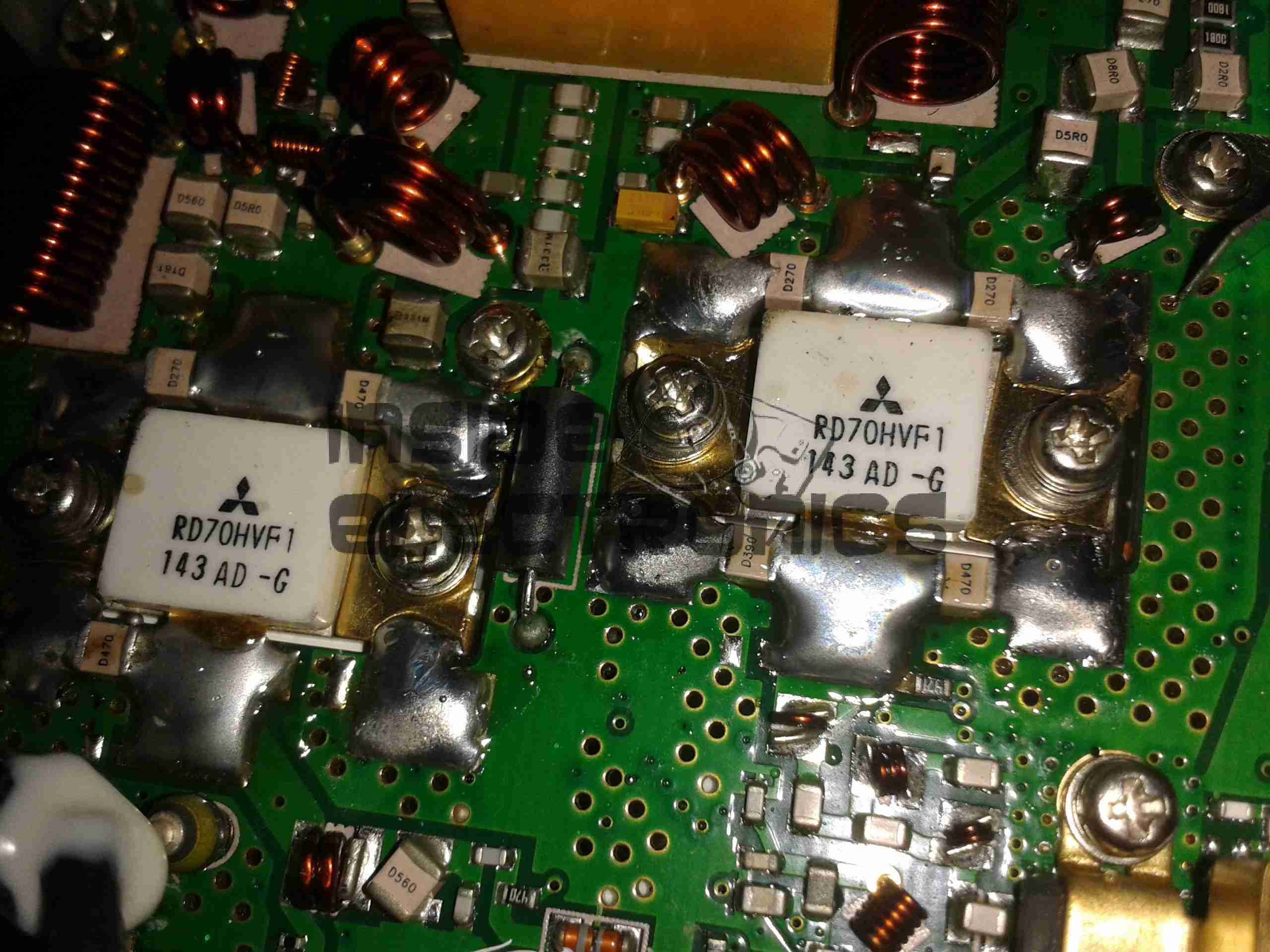
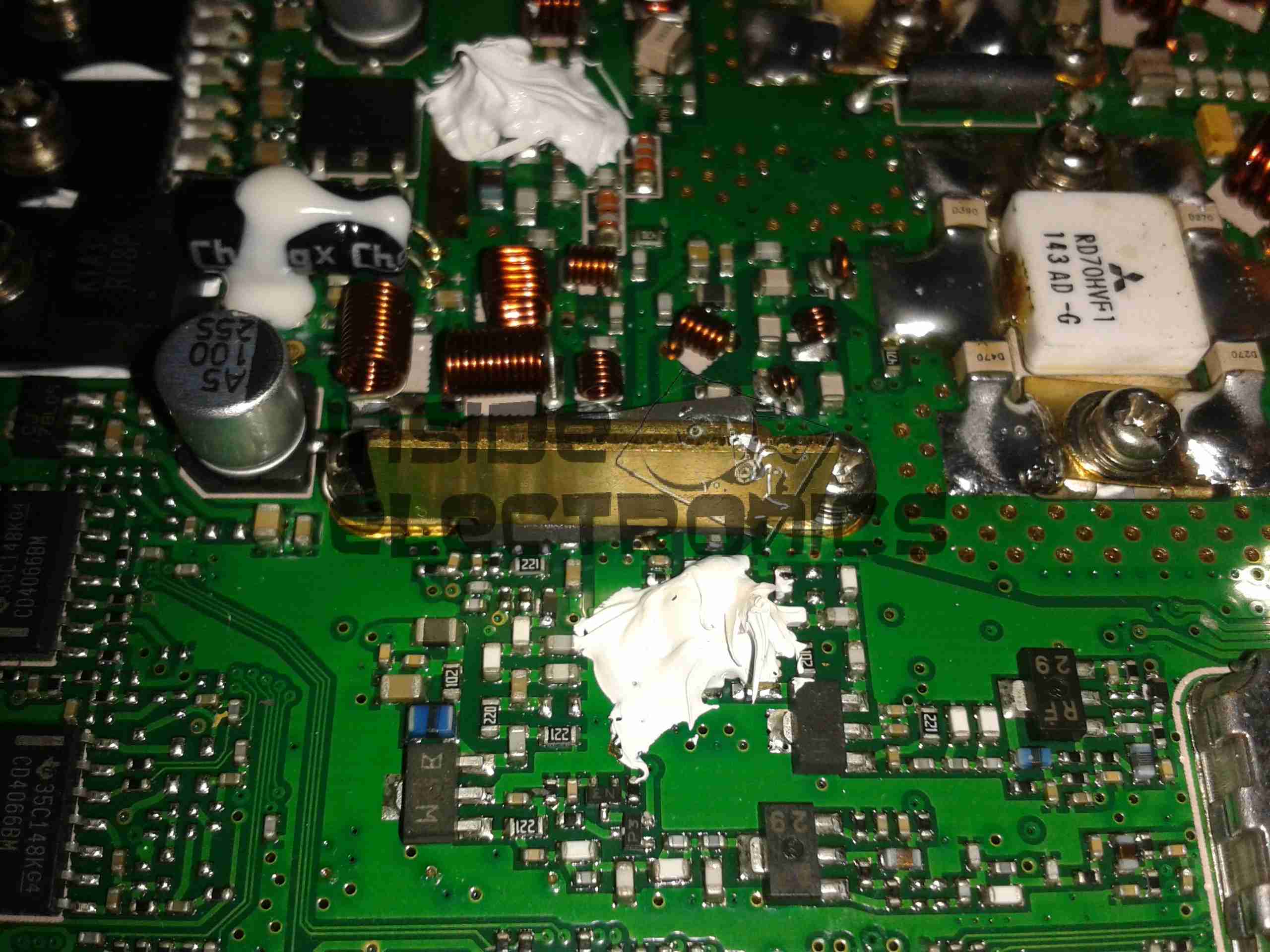
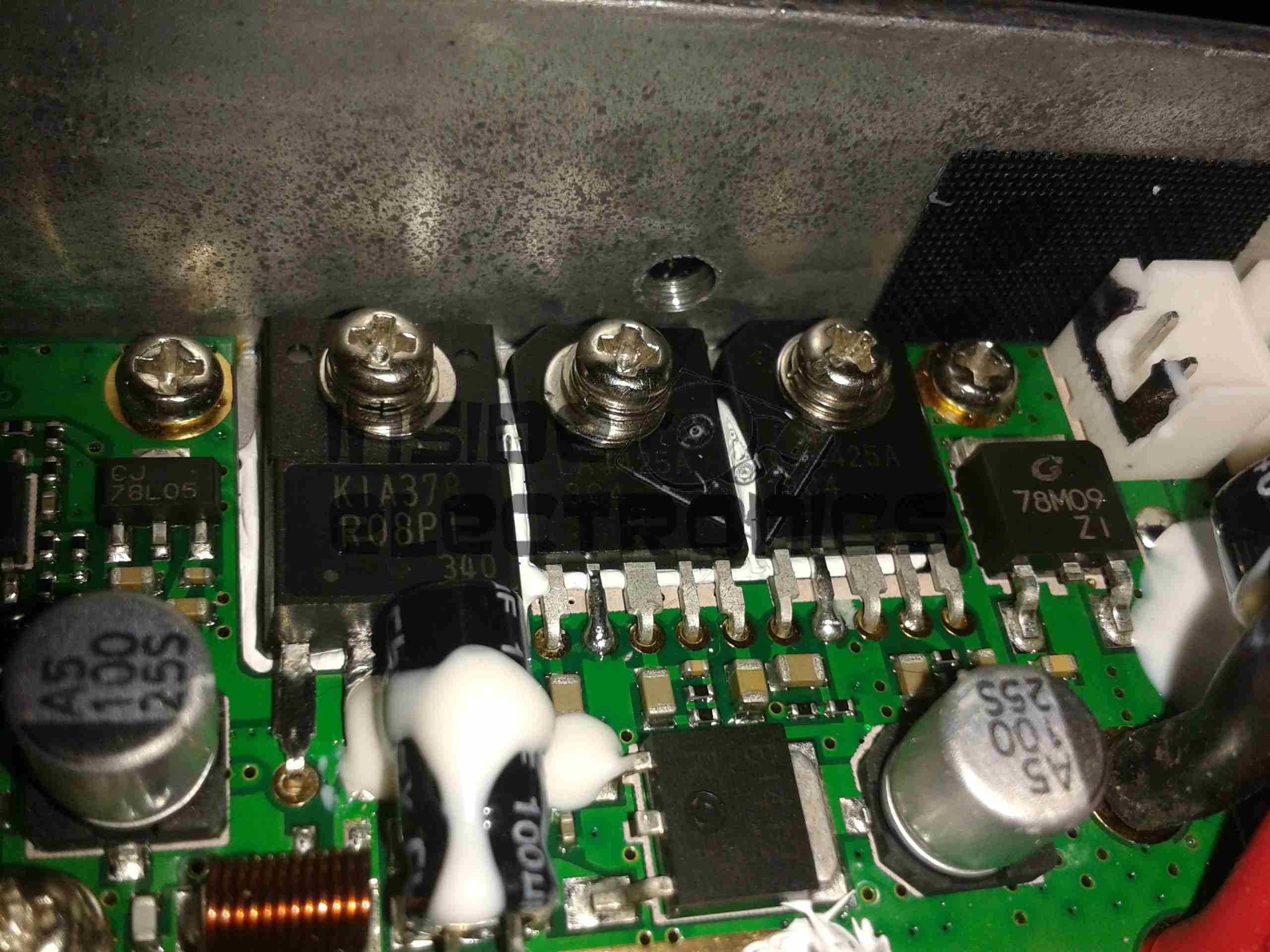
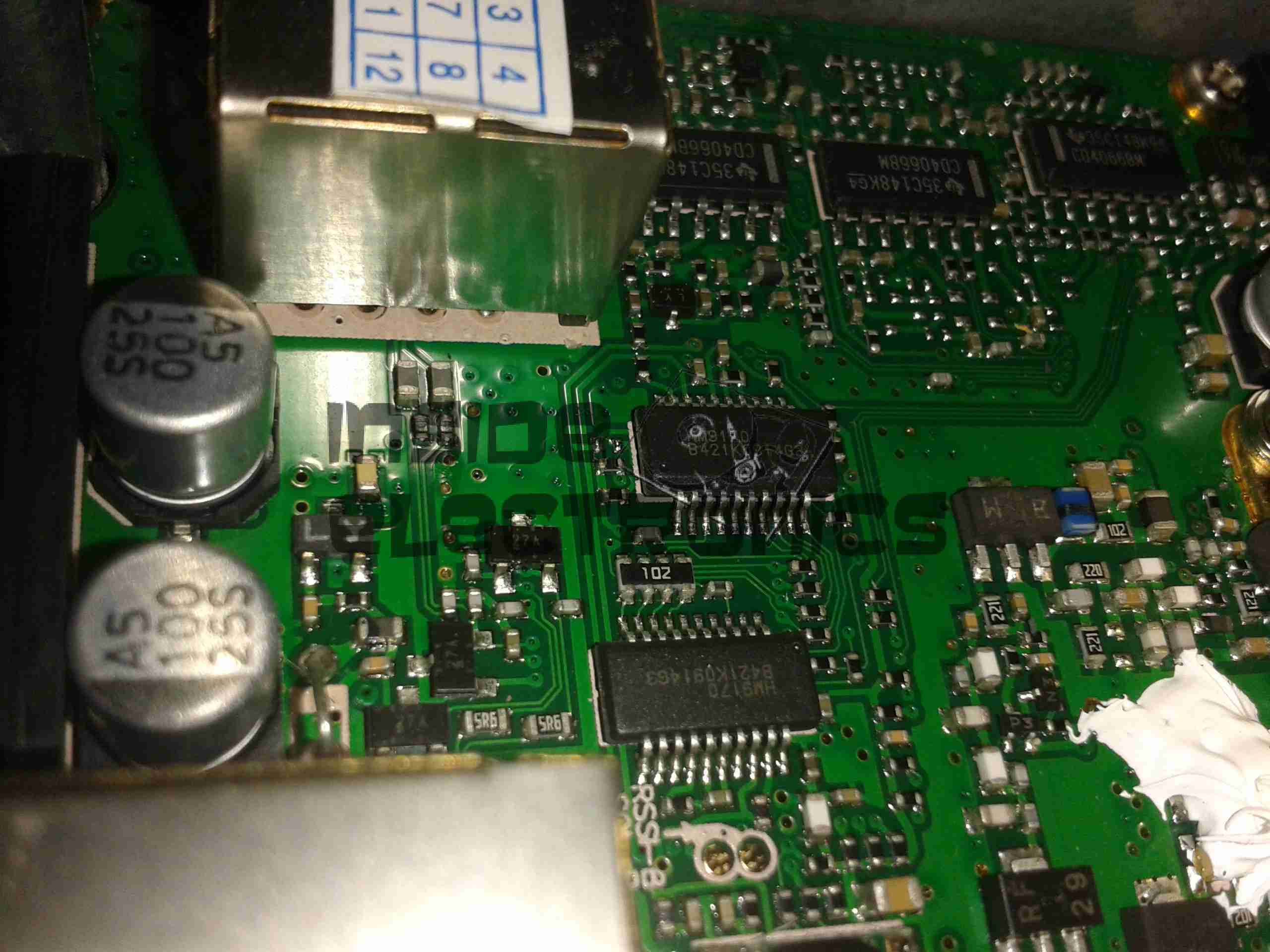
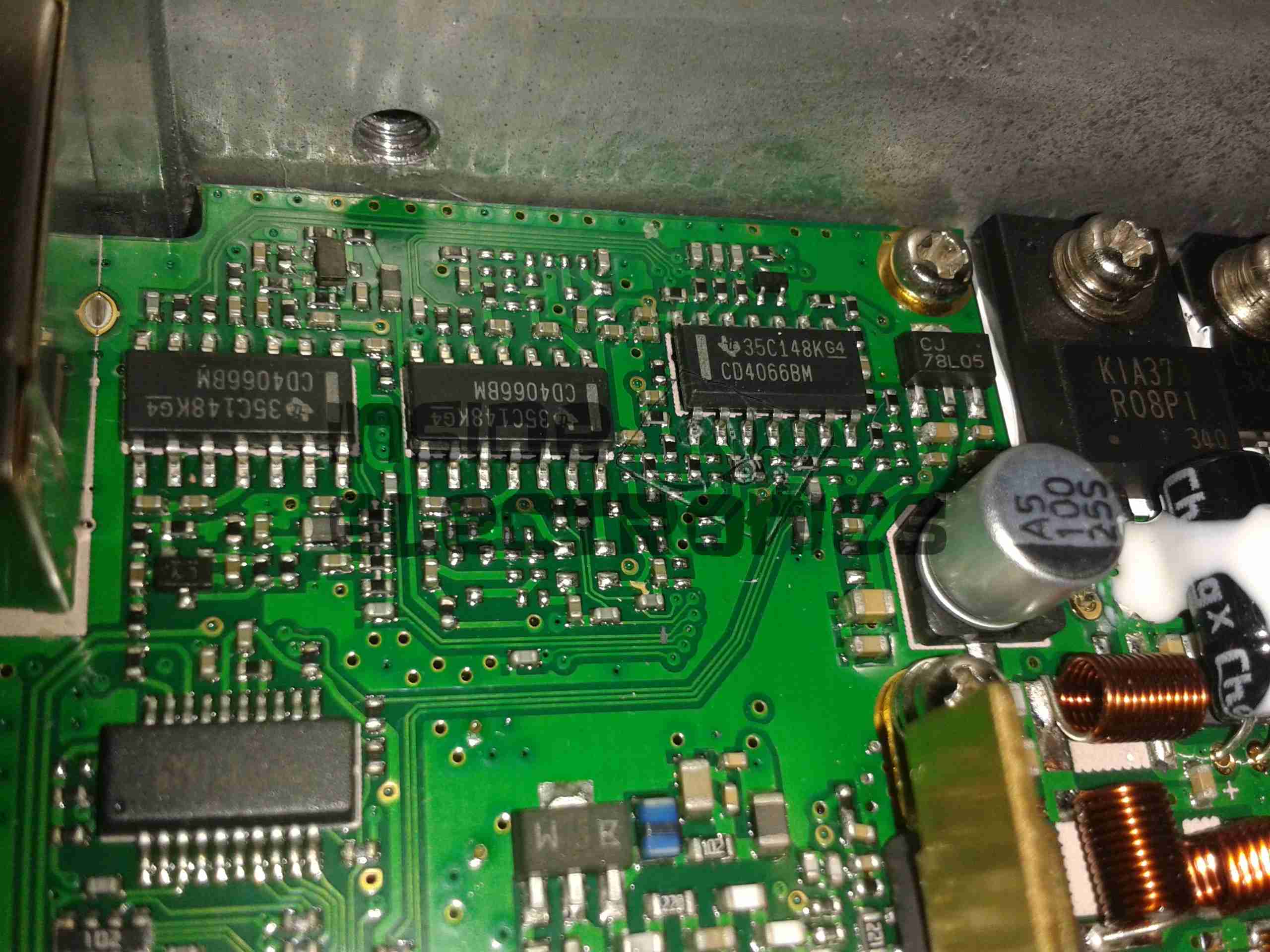
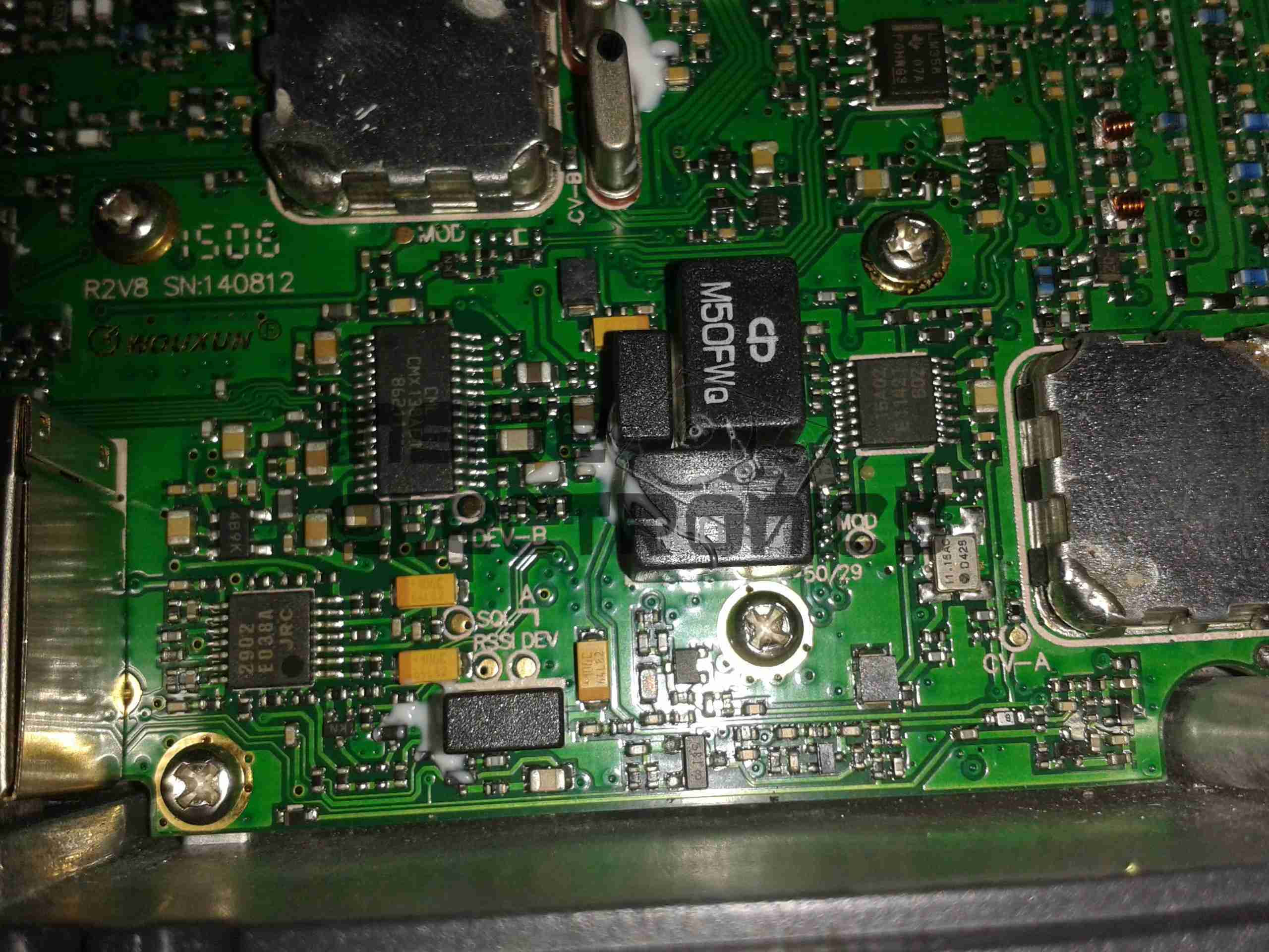
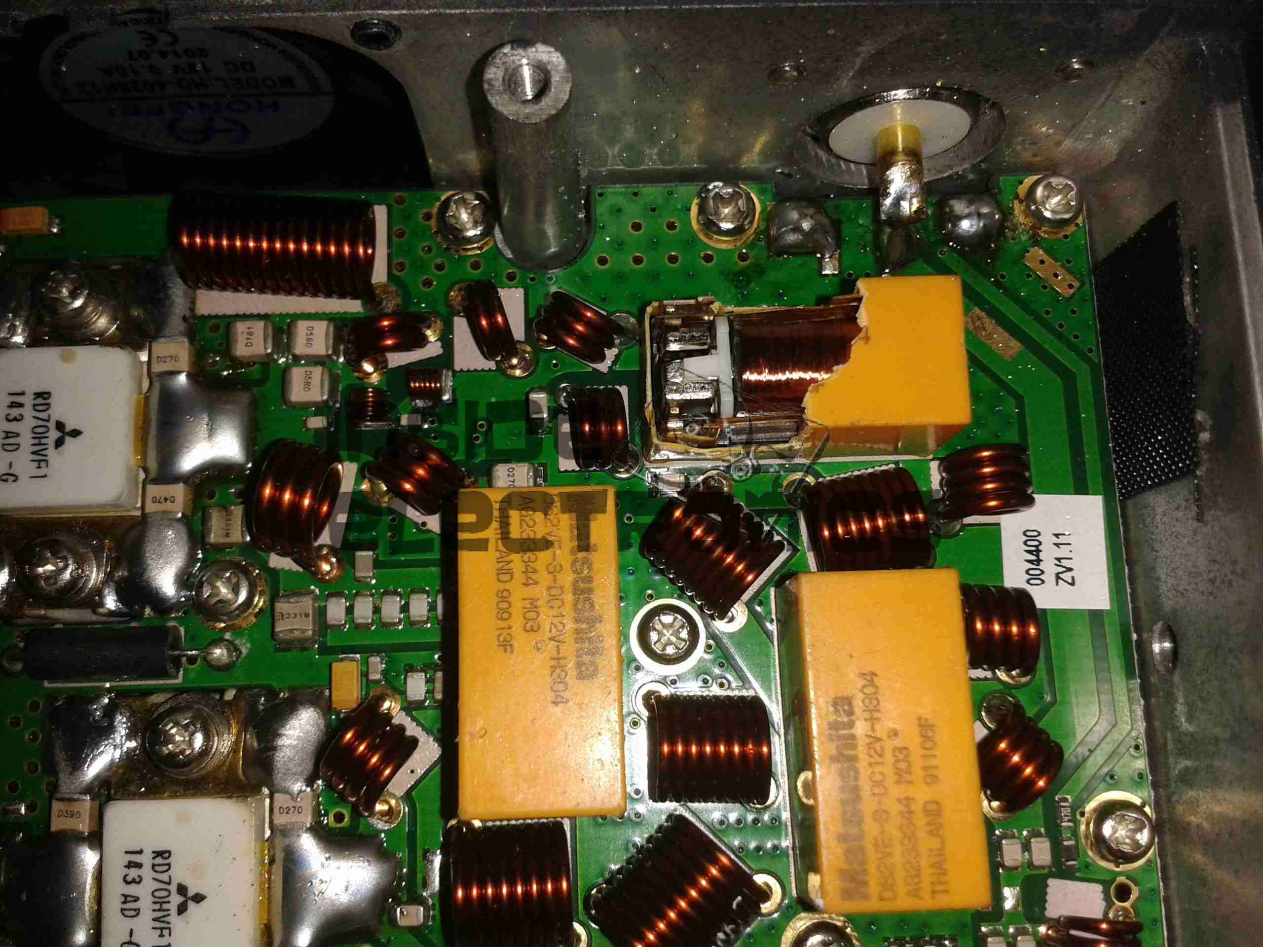
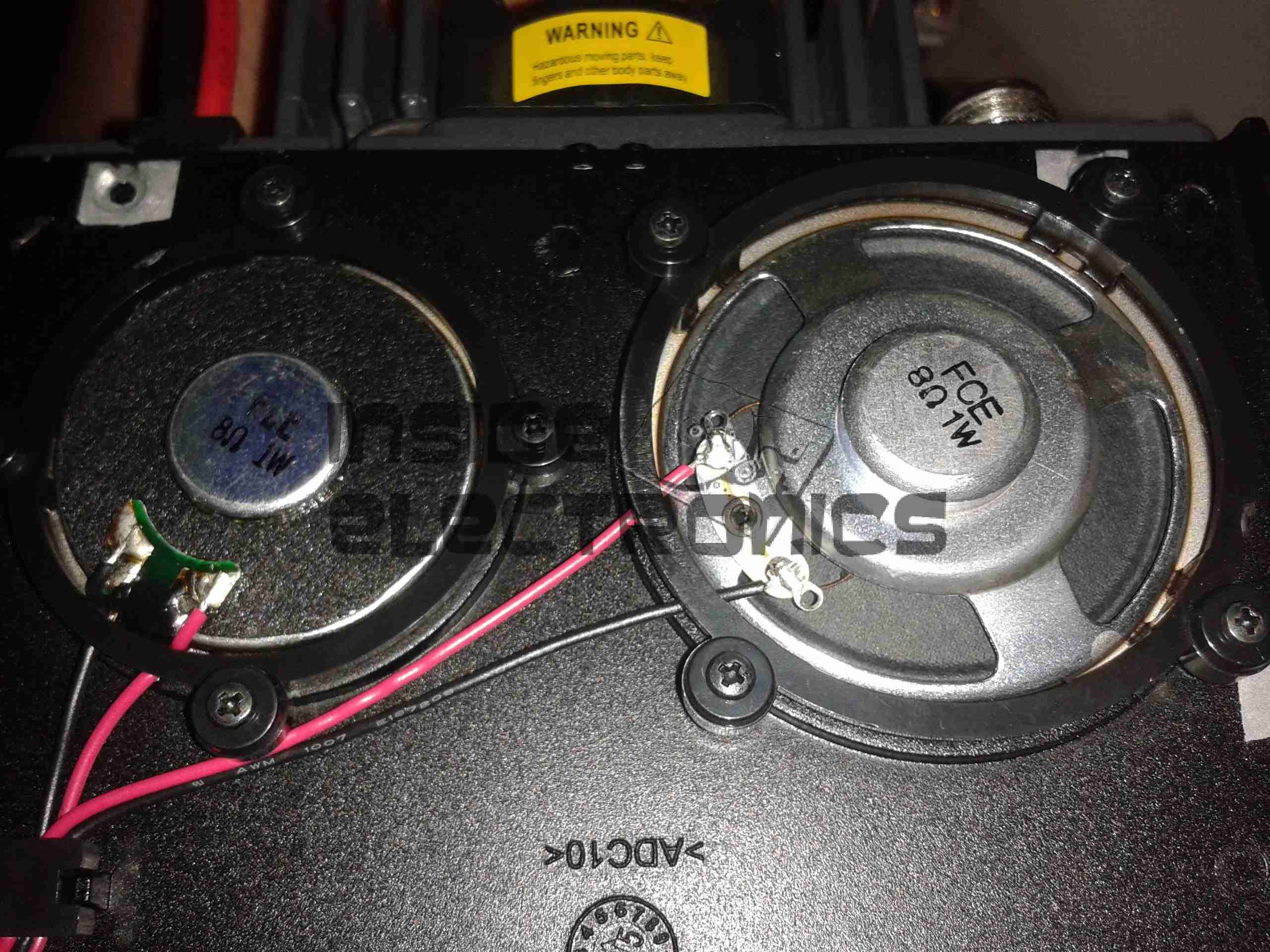
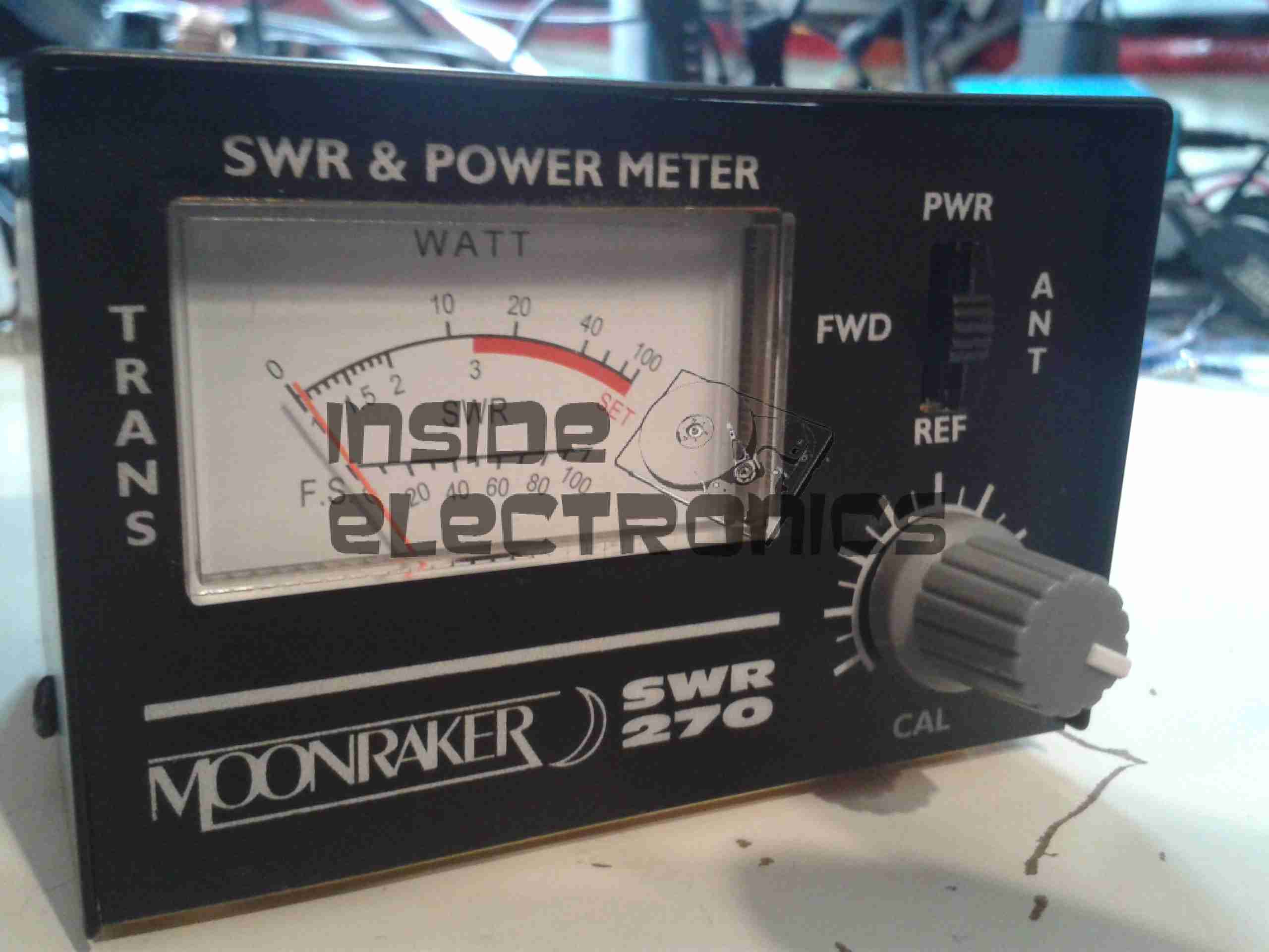
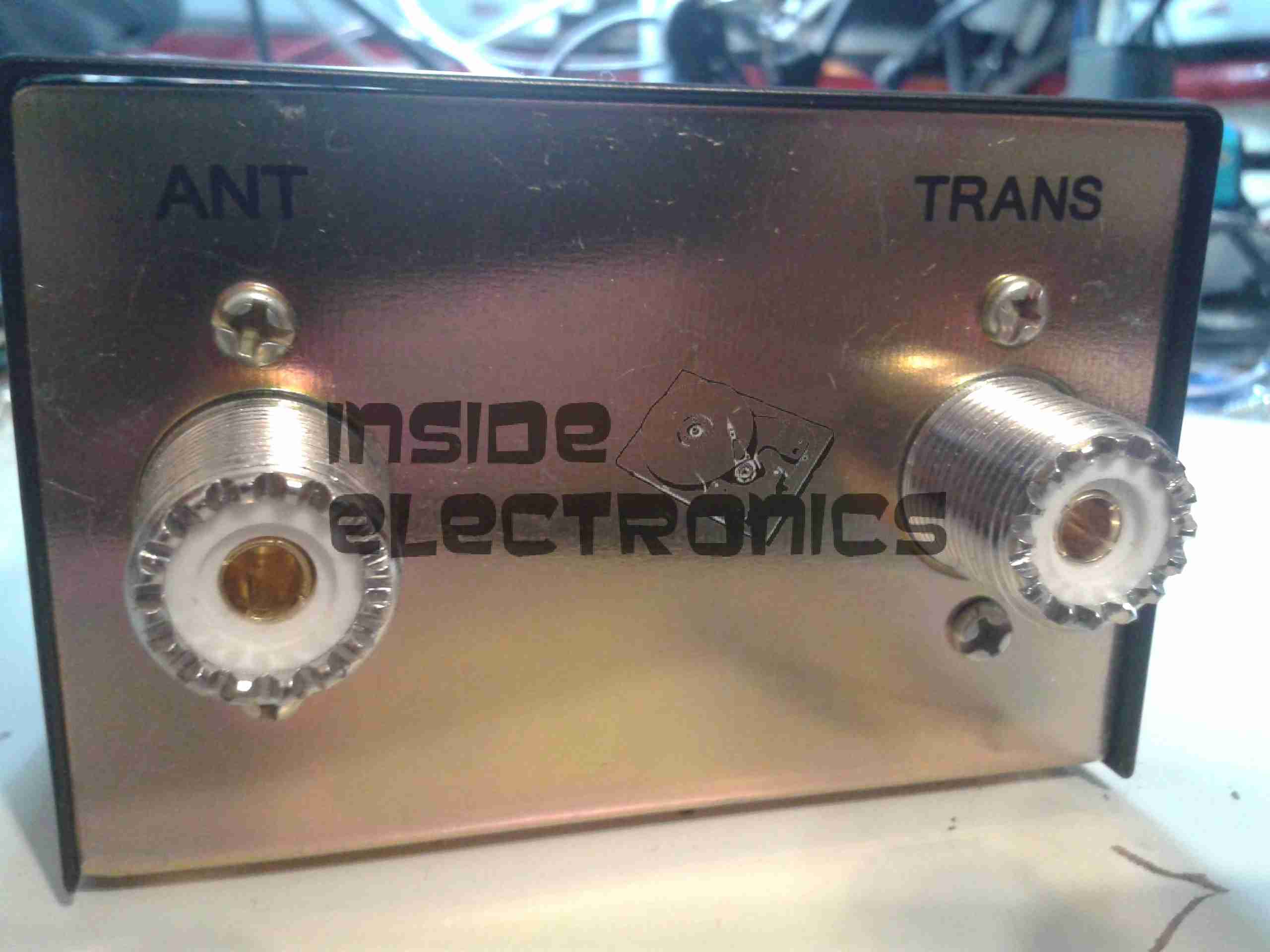
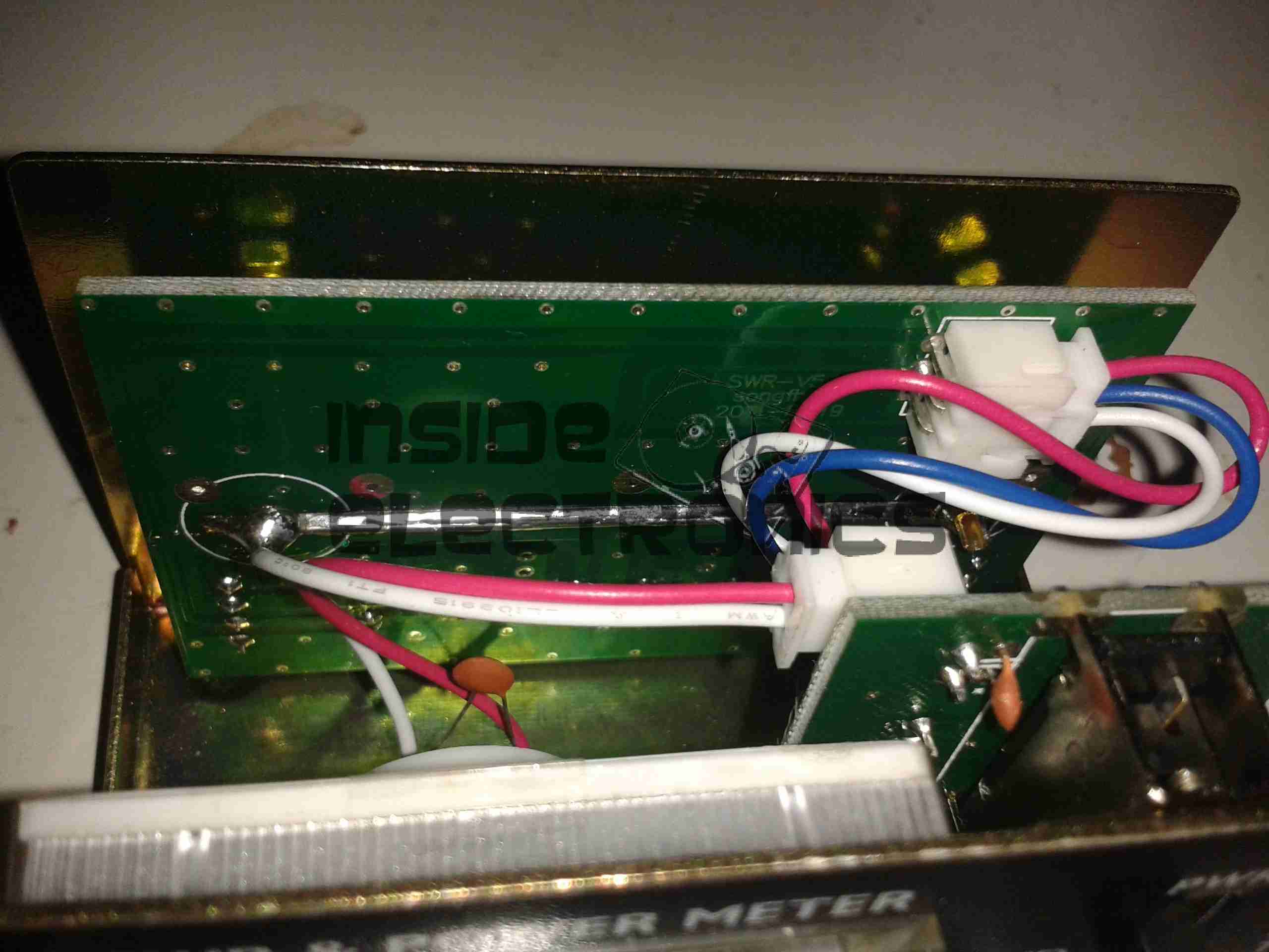

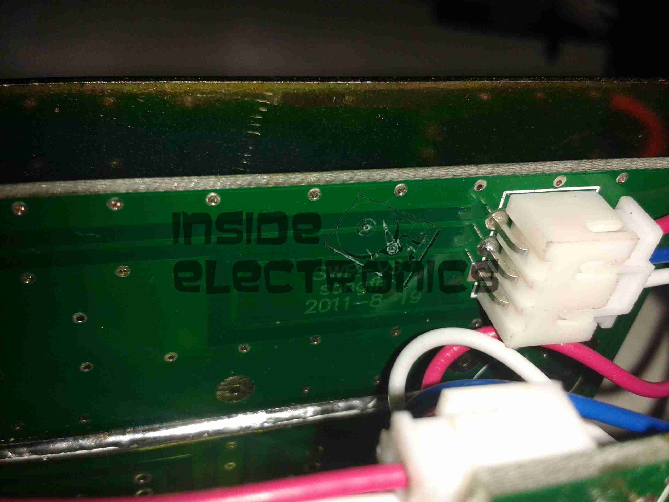
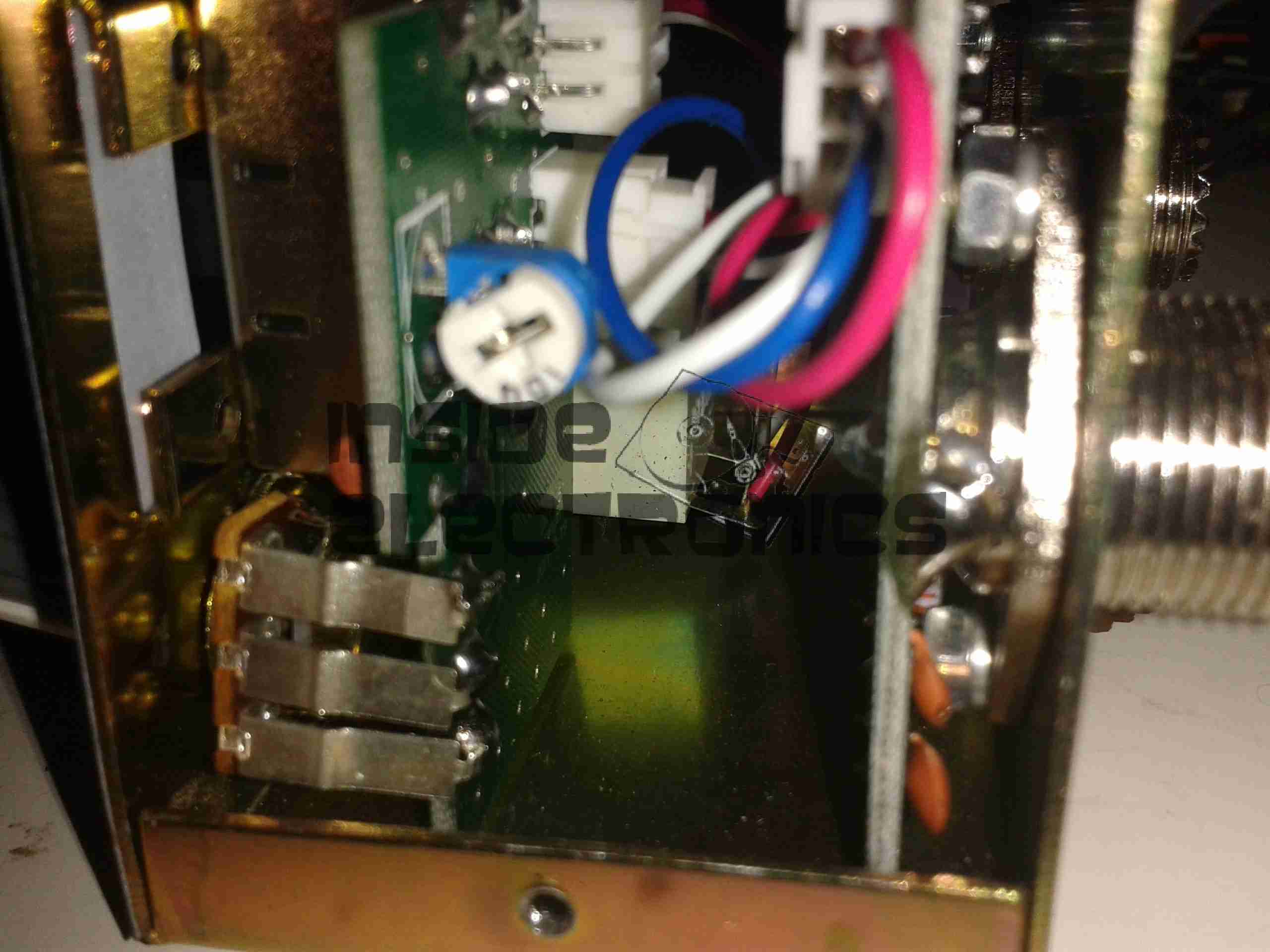
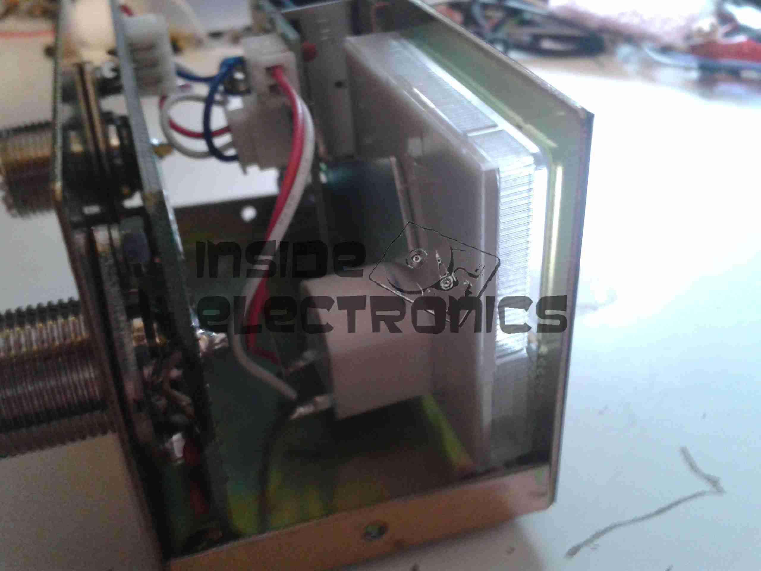
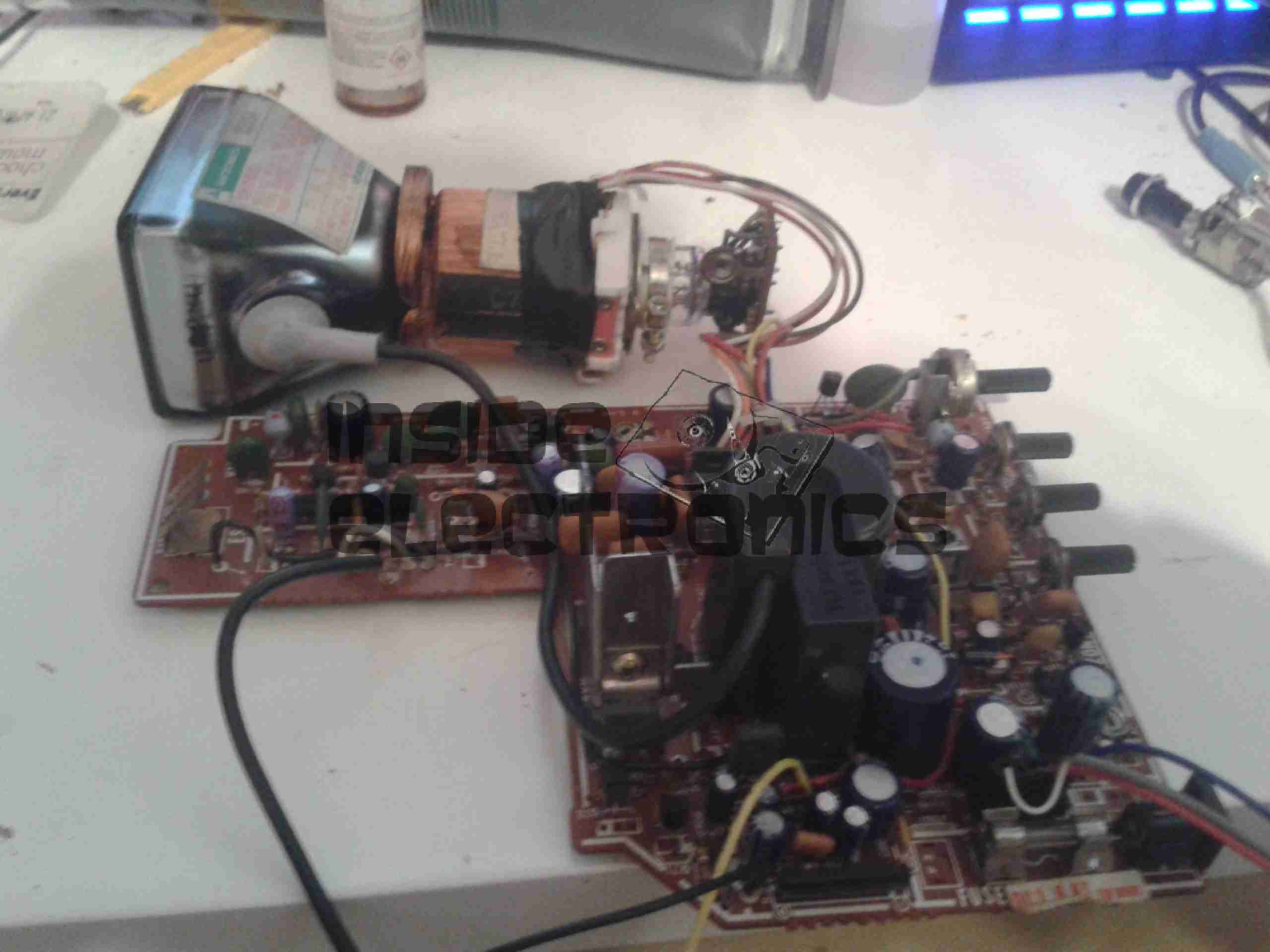
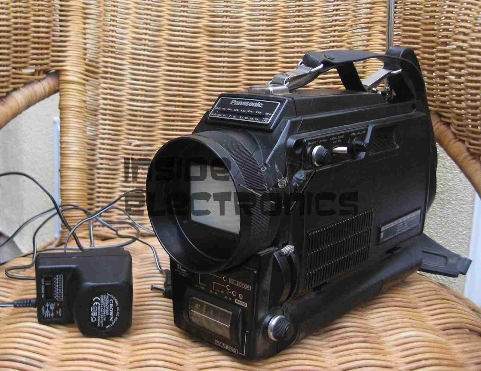
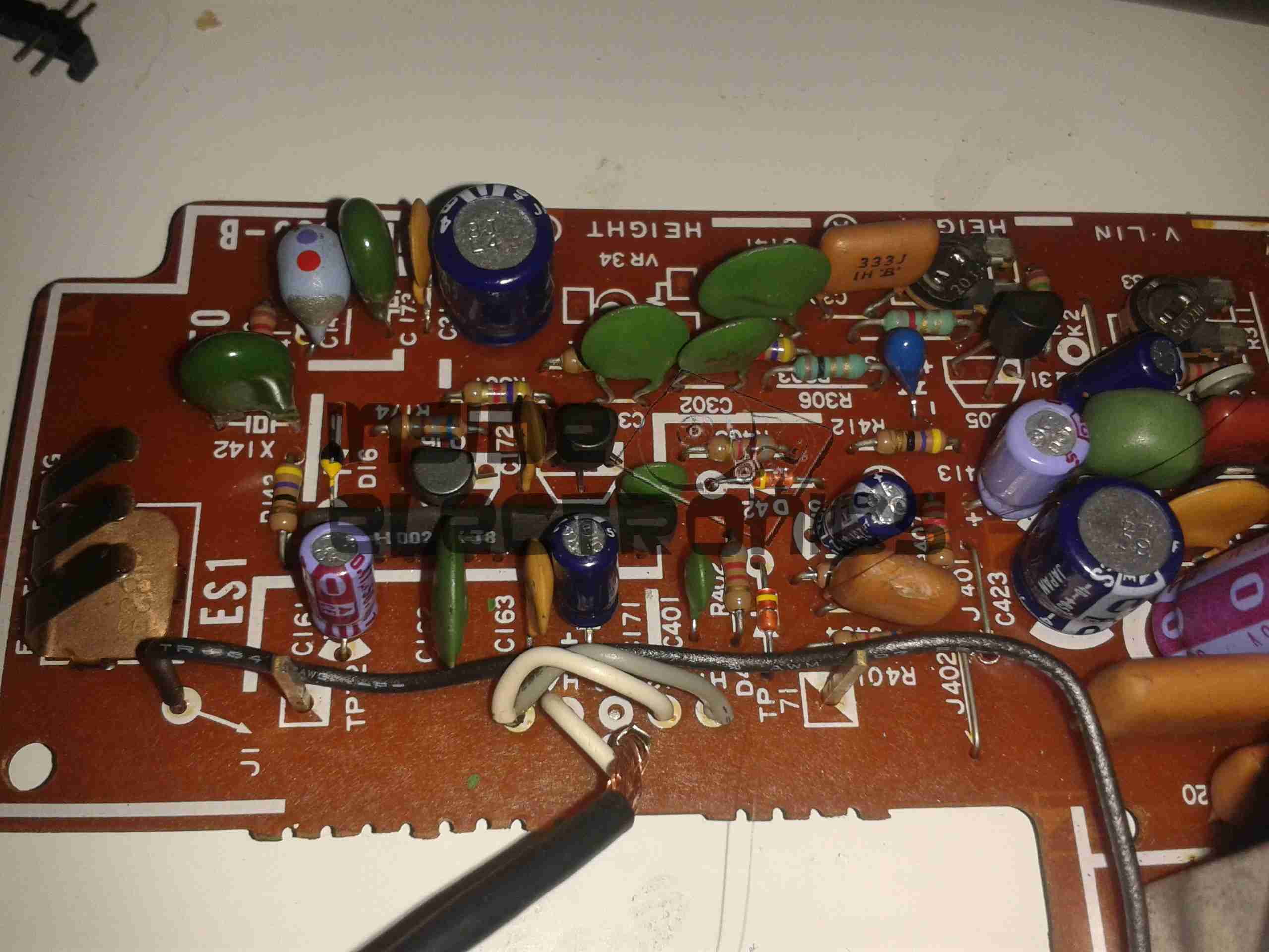
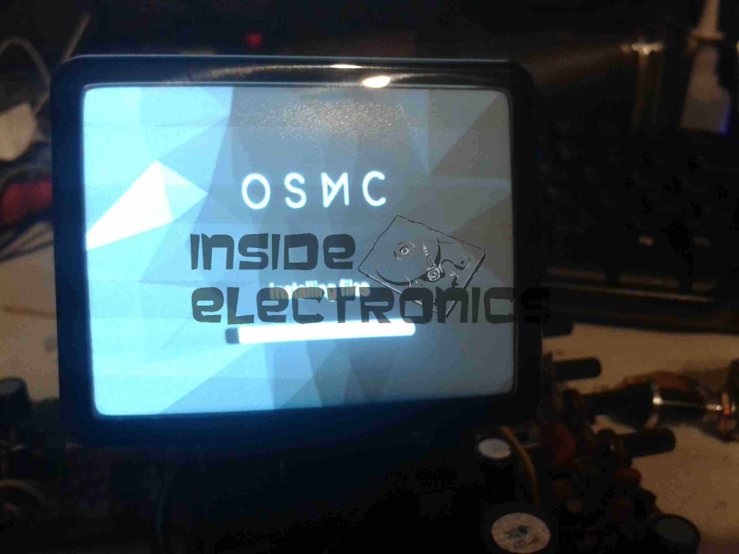
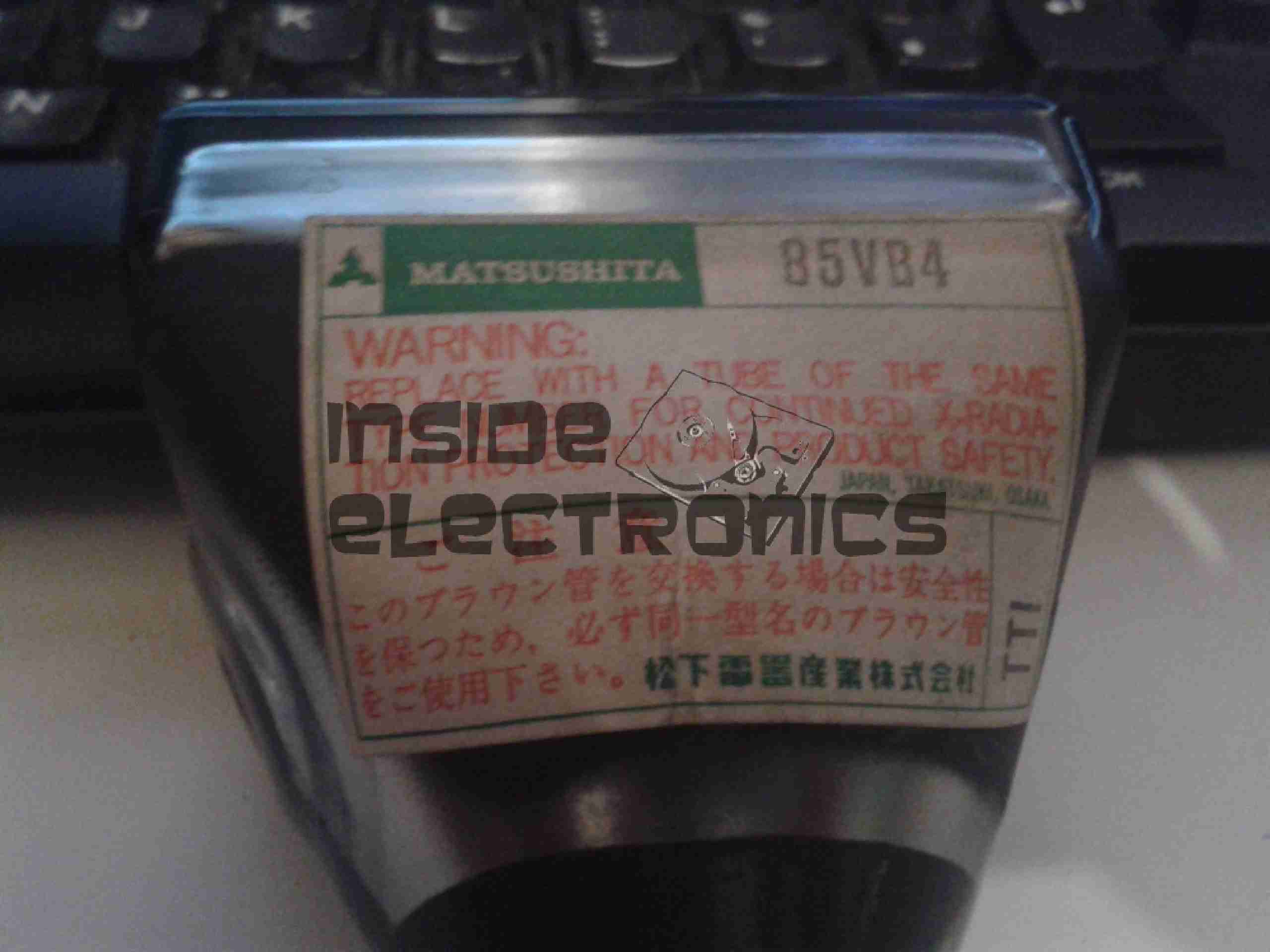
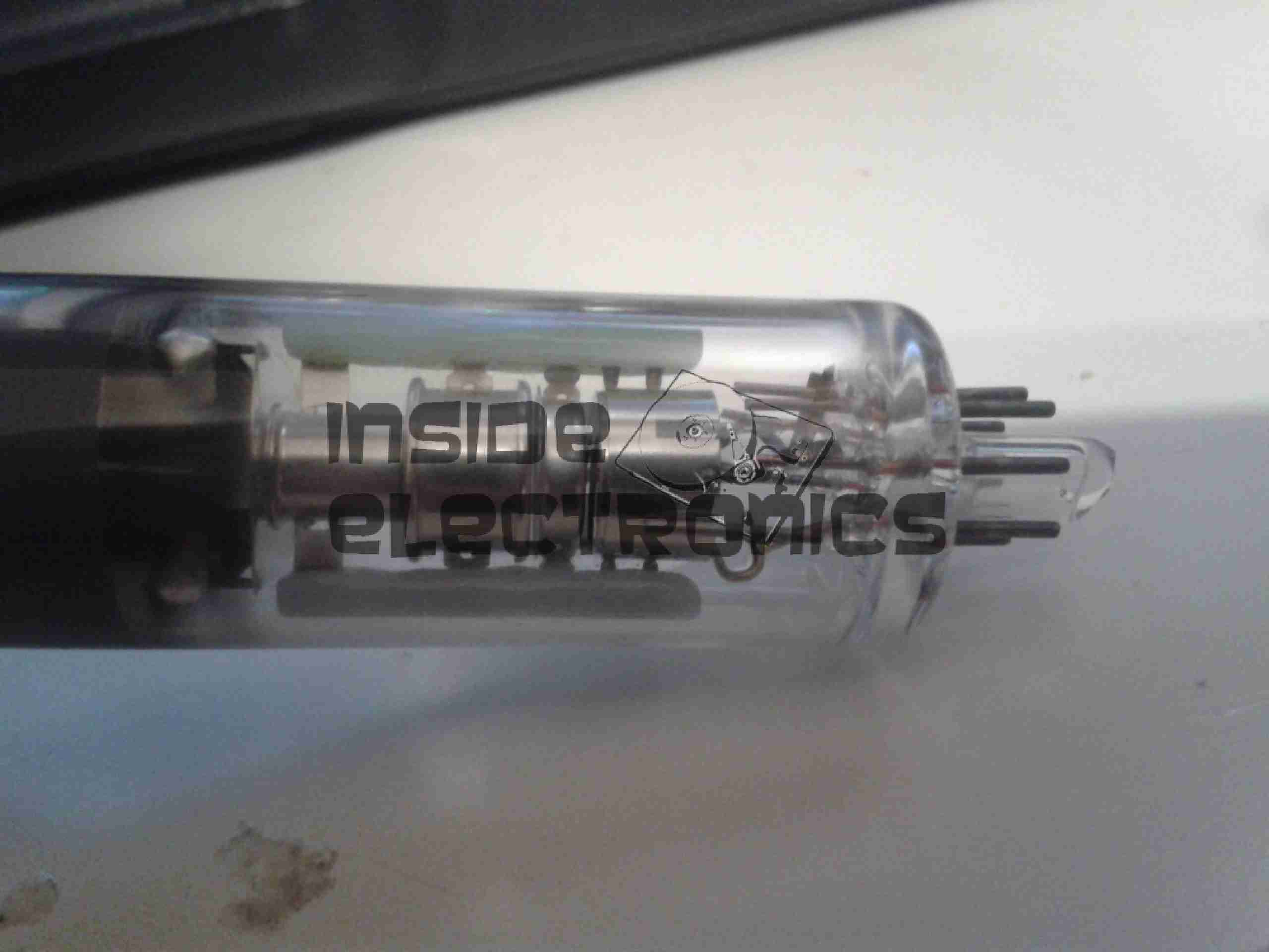
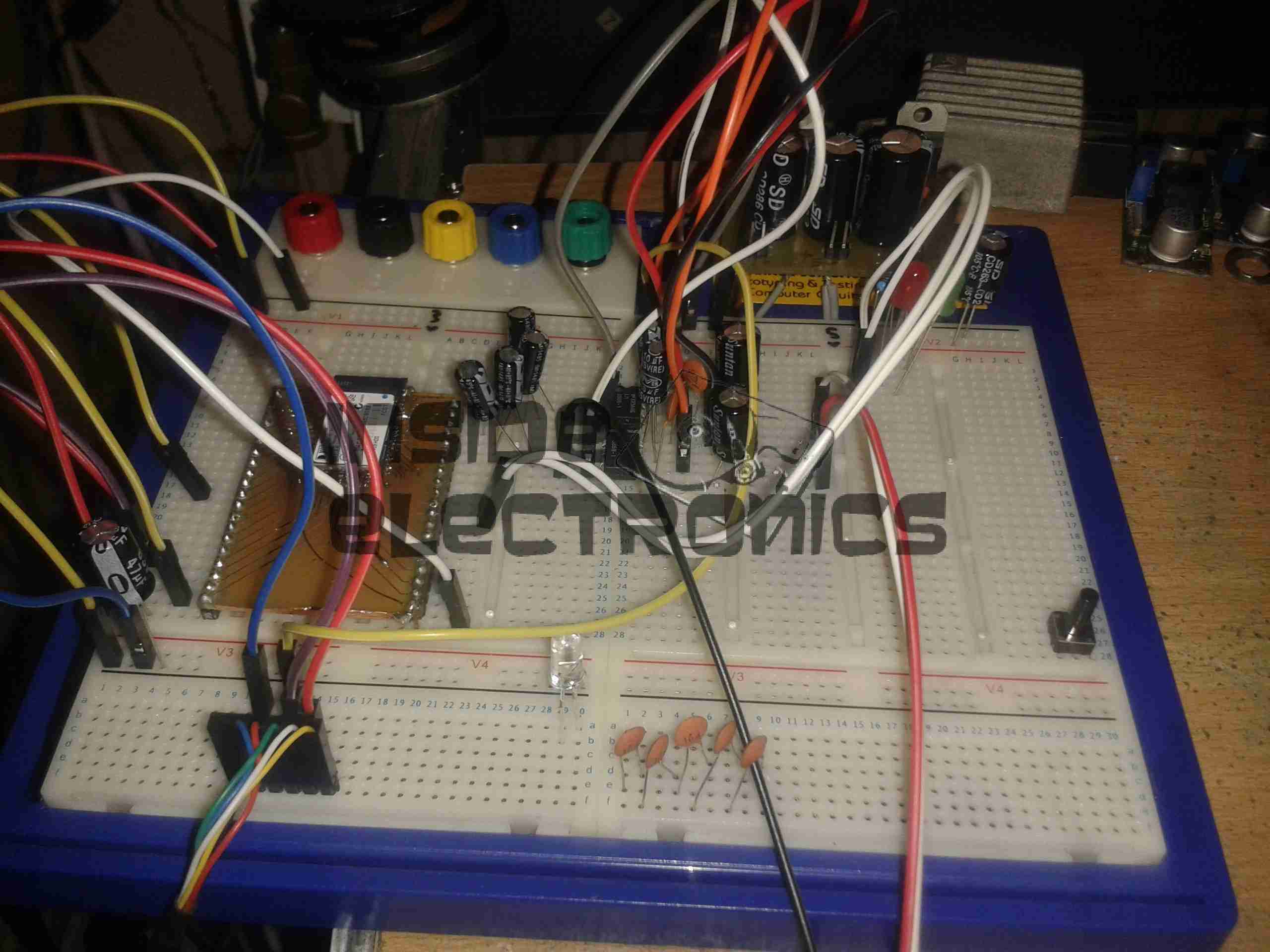
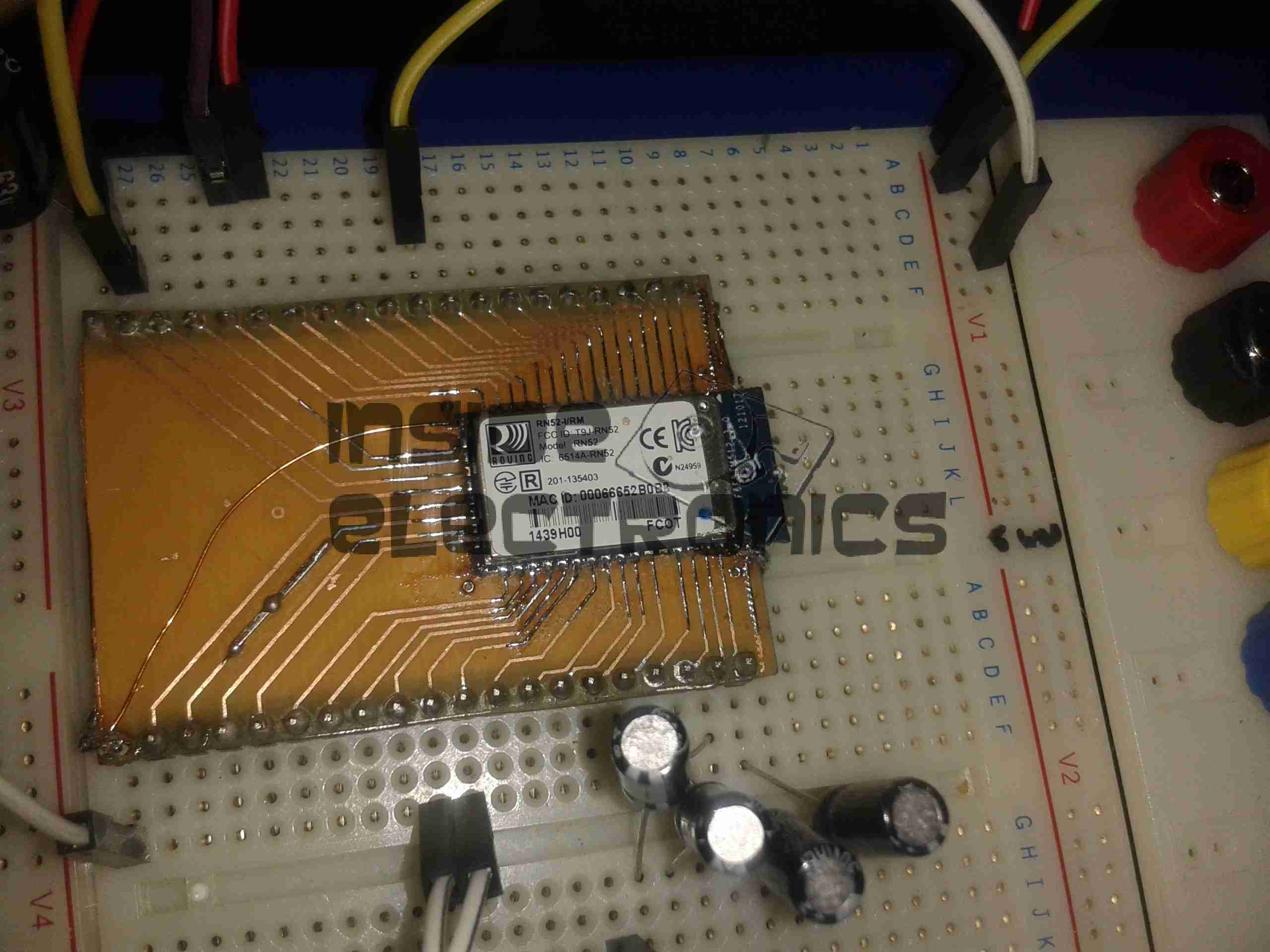
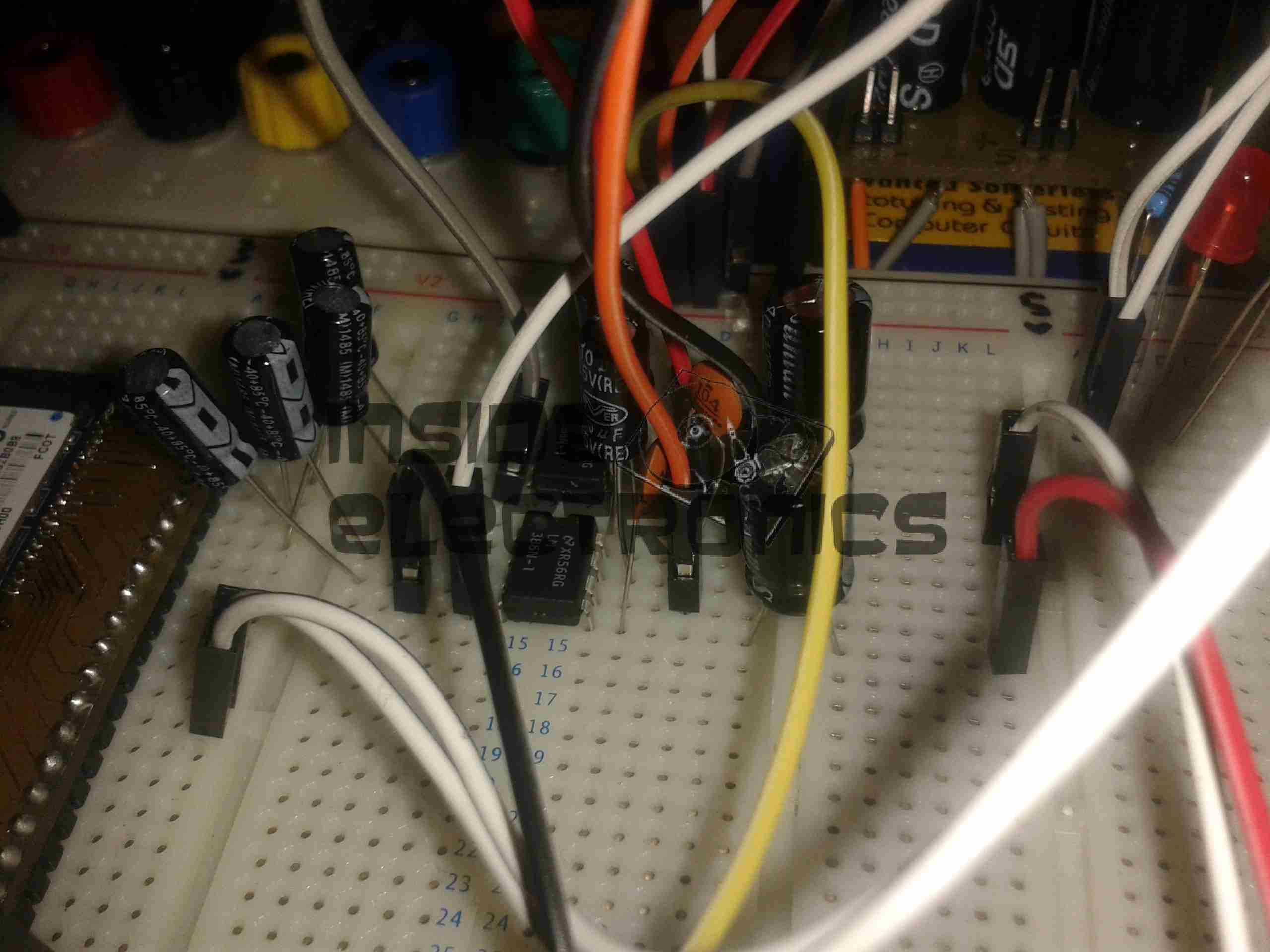
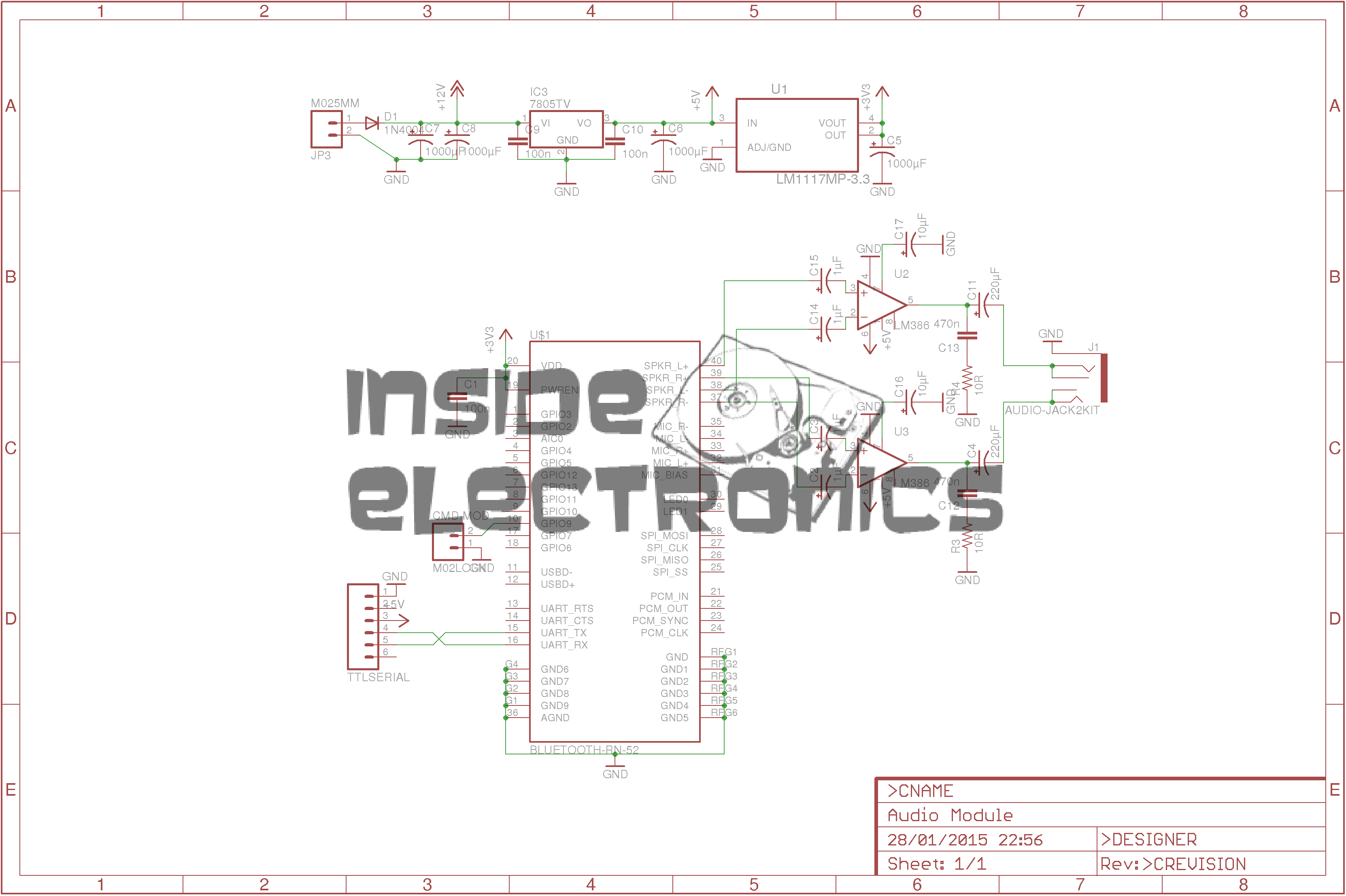
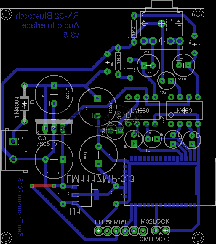
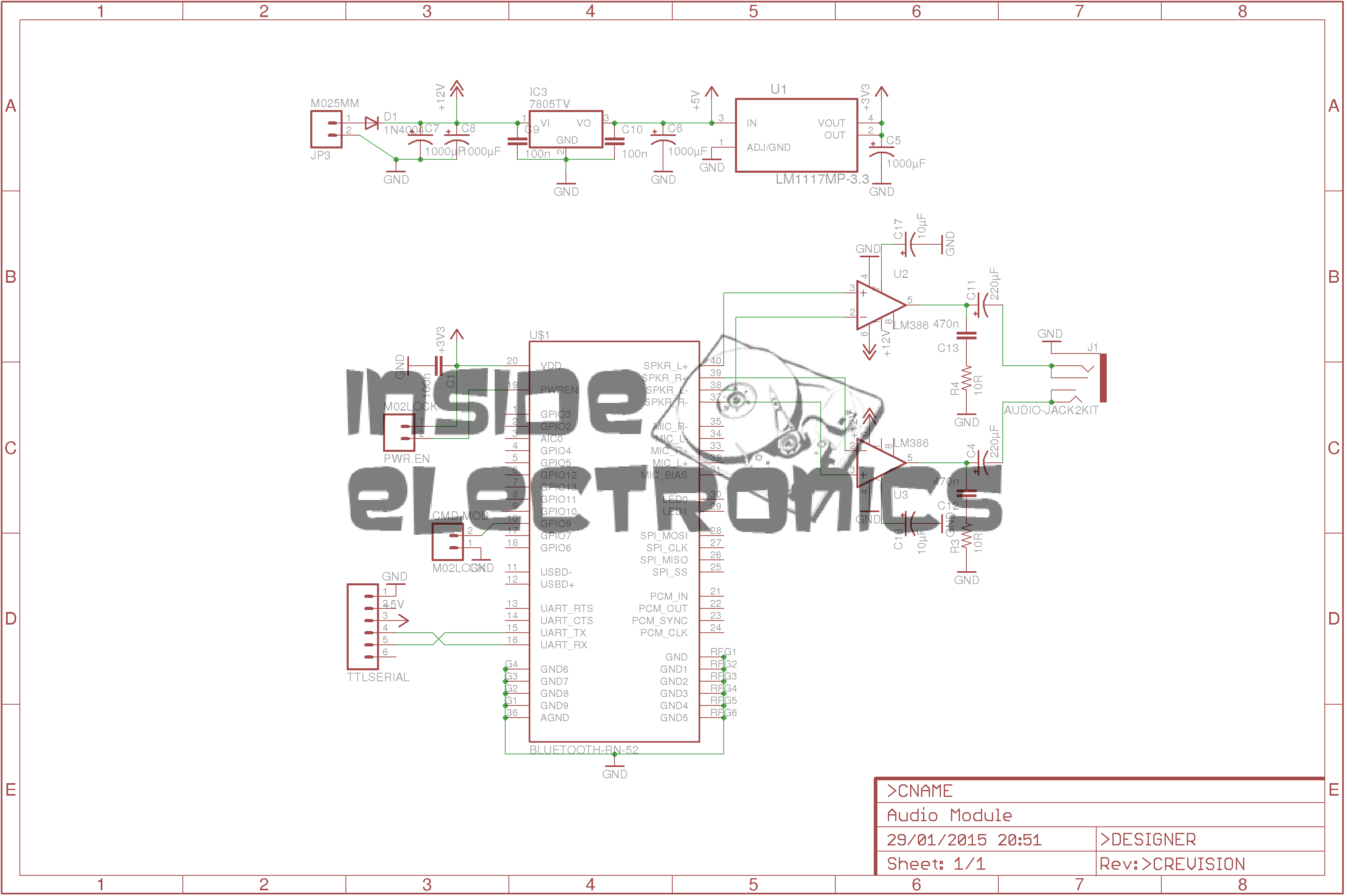
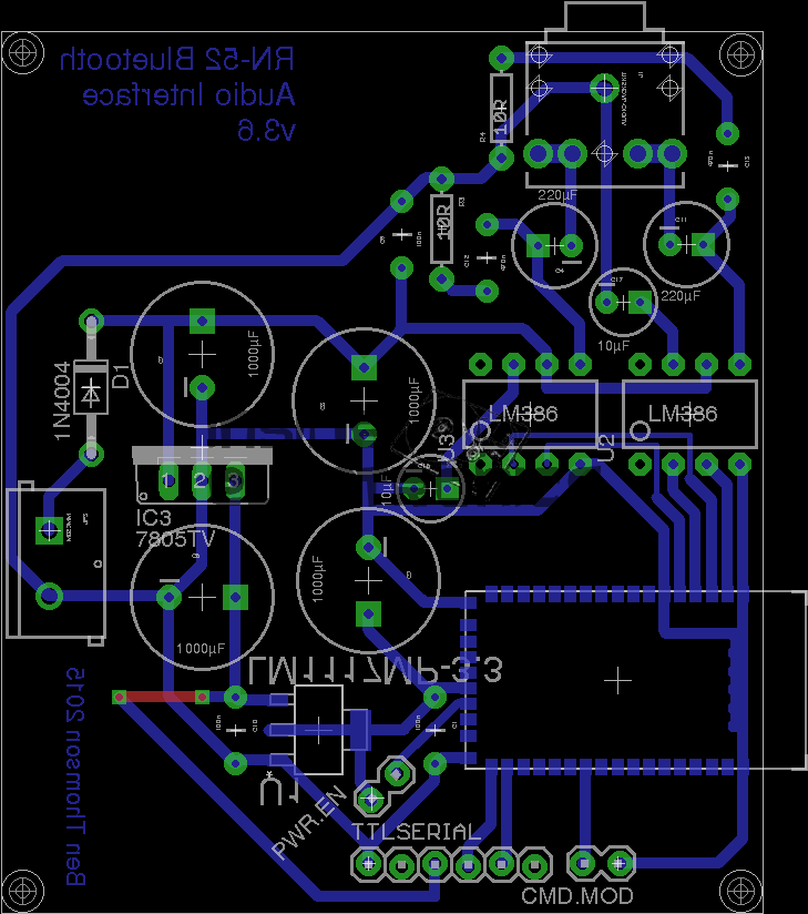
